Сортировка кучей, пирамидальная сортировка (англ. Heapsort) — алгоритм сортировки, использующий структуру данных двоичная куча. Это неустойчивый алгоритм сортировки с временем работы , где — количество элементов для сортировки, и использующий дополнительной памяти.
Содержание
- 1 Алгоритм
- 2 Реализация
- 3 Сложность
- 4 Пример
- 5 JSort
- 5.1 Алгоритм
- 5.2 Сложность
- 5.3 Пример
- 5.4 См. также
- 5.5 Источники информации
Алгоритм
Необходимо отсортировать массив , размером . Построим на базе этого массива за кучу для максимума. Так как максимальный элемент находится в корне, то если поменять его местами с , он встанет на своё место. Далее вызовем процедуру , предварительно уменьшив на . Она за просеет на нужное место и сформирует новую кучу (так как мы уменьшили её размер, то куча располагается с по , а элемент находится на своём месте). Повторим эту процедуру для новой кучи, только корень будет менять местами не с , а с . Делая аналогичные действия, пока не станет равен , мы будем ставить наибольшее из оставшихся чисел в конец не отсортированной части. Очевидно, что таким образом, мы получим отсортированный массив.
Реализация
- — массив, который необходимо отсортировать
- — количество элементов в нём
- — процедура, которая строит из передаваемого массива кучу для максимума в этом же массиве
- — процедура, которая просеивает вниз элемент в куче из элементов, находящихся в начале массива
 fun heapSort(A : list <T>):
   buildHeap(A)
   heapSize = A.size
   for i = 0 to n - 1
     swap(A[0], A[n - 1 - i])
     heapSize--
     siftDown(A, 0, heapSize)
Сложность
Операция работает за . Всего цикл выполняется раз. Таким образом сложность сортировки кучей является .
Достоинства:
- худшее время работы — ,
- требует дополнительной памяти.
Недостатки:
- неустойчивая,
- на почти отсортированных данных работает столь же долго, как и на хаотических данных.
Пример
|
|
|
|
|
|
|
|


Пусть дана последовательность из элементов .
| Массив | Описание шага |
|---|---|
| 5 3 4 1 2 | Строим кучу из исходного массива |
| Первый проход | |
| 2 3 4 1 5 | Меняем местами первый и последний элементы |
| 4 3 2 1 5 | Строим кучу из первых четырёх элементов |
| Второй проход | |
| 1 3 2 4 5 | Меняем местами первый и четвёртый элементы |
| 3 1 2 4 5 | Строим кучу из первых трёх элементов |
| Третий проход | |
| 2 1 3 4 5 | Меняем местами первый и третий элементы |
| 2 1 3 4 5 | Строим кучу из двух элементов |
| Четвёртый проход | |
| 1 2 3 4 5 | Меняем местами первый и второй элементы |
| 1 2 3 4 5 | Массив отсортирован |
JSort
JSort является модификацией сортировки кучей, которую придумал Джейсон Моррисон (Jason Morrison).
Алгоритм частично упорядочивает массив, строя на нём два раза кучу: один раз передвигая меньшие элементы влево, второй раз передвигая большие элементы вправо. Затем к массиву применяется
сортировка вставками, которая при почти отсортированных данных работает за .
Достоинства:
- В отличие от сортировки кучей, на почти отсортированных массивах работает быстрее, чем на случайных.
- В силу использования сортировки вставками, которая просматривает элементы последовательно, использование кэша гораздо эффективнее.
Недостатки:
- На длинных массивах, возникают плохо отсортированные последовательности в середине массива, что приводит к ухудшению работы сортировки вставками.
Алгоритм
Построим кучу для минимума на этом массиве.
Тогда наименьший элемент окажется на первой позиции, а левая часть массива окажется почти отсортированной, так как ей будут соответствовать верхние узлы кучи.
Теперь построим на этом же массиве кучу так, чтобы немного упорядочить правую часть массива. Эта куча должна быть кучей для максимума и быть «зеркальной» к массиву, то есть чтобы её корень соответствовал последнему элементу массива.
К получившемуся массиву применим сортировку вставками.
Сложность
Построение кучи занимает . Почти упорядоченный массив сортировка вставками может отсортировать , но в худшем случае за .
Таким образом, наихудшая оценка Jsort — .
Пример
Рассмотрим, массив =
Построим на этом массиве кучу для минимума:
Массив выглядит следующим образом:
![]()
Заметим, что начало почти упорядочено, что хорошо скажется на использовании сортировки вставками.
Построим теперь зеркальную кучу для максимума на этом же массиве.
Массив будет выглядеть следующим образом:
![]()
Теперь и конец массива выглядит упорядоченным, применим сортировку вставками и получим отсортированный массив.
См. также
- Сортировка слиянием
- Быстрая сортировка
- Теорема о нижней оценке для сортировки сравнениями
Источники информации
- Кормен Т., Лейзерсон Ч., Ривест Р., Штайн К. Алгоритмы: построение и анализ, 2-е издание. Издательский дом «Вильямс», 2005. ISBN 5-8459-0857-4
- Wikipedia — Heapsort
- Wikipedia — JSort
- Хабрахабр — Описание сортировки кучей и JSort
- Википедия — Пирамидальная сортировка
- 1. Что такое бинарное дерево? Какие виды бинарных деревьев существуют?
- 2. Как создать полное бинарное дерево из несортированного списка (массива)?
- 3. Связь между индексами массива и элементами дерева
- 4. Что такое структура данных кучи?
- 5. Как выстроить дерево
- 6. Сборка убывающей кучи
- 7. Процедуры для Heapsort
- 8. Представление
- 9. Применение сортировки кучей
- 10. Реализация сортировки кучи на разных языках программирования
Сортировка кучей — популярный и эффективный алгоритм сортировки в компьютерном программировании. Чтобы научиться писать алгоритм сортировки кучей, требуется знание двух типов структур данных — массивов и деревьев.
Например, начальный набор чисел, которые мы хотим отсортировать, хранится в массиве [10, 3, 76, 34, 23, 32], и после сортировки мы получаем отсортированный массив [3,10,23,32,34,76].
Сортировка кучей работает путем визуализации элементов массива как особого вида полного двоичного дерева, называемого кучей.
Что такое бинарное дерево? Какие виды бинарных деревьев существуют?
Бинарное дерево
— это структура данных дерева, в которой каждый родительский узел может иметь не более двух дочерних элементов.

Полное бинарное дерево
— это особый тип бинарного дерева, в котором у каждого родительского узла есть два или нет дочерних элементов.

Идеальное бинарное дерево
похоже на полное бинарное дерево, но с двумя основными отличиями:
- Каждый уровень должен быть полностью заполнен.
- Все элементы листа должны наклоняться влево.
Примечание: Последний элемент может не иметь правильного брата, то есть идеальное бинарное дерево не обязательно должно быть полным бинарным деревом.

Как создать полное бинарное дерево из несортированного списка (массива)?
- Выберите первый элемент списка, чтобы он быть корневым узлом. (Первый уровень — 1 элемент).
- Поместите второй элемент в качестве левого дочернего элемента корневого узла, а третий элемент — в качестве правого дочернего элемента. (Второй уровень — 2 элемента).
- Поместите следующие два элемента в качестве дочерних элементов левого узла второго уровня. Снова, поместите следующие два элемента как дочерние элементы правого узла второго уровня (3-й уровень — 4 элемента).
- Продолжайте повторять, пока не дойдете до последнего элемента.

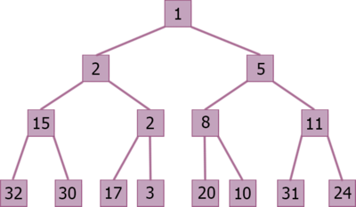
Связь между индексами массива и элементами дерева
Полное бинарное дерево обладает интересным свойством, которое мы можем использовать для поиска дочерних элементов и родителей любого узла.
Если индекс любого элемента в массиве равен i, элемент в индексе 2i + 1 станет левым потомком, а элемент в индексе 2i + 2 станет правым потомком. Кроме того, родительский элемент любого элемента с индексом i задается нижней границей (i-1) / 2.

Проверим это:
Left child of 1 (index 0) = element in (2*0+1) index = element in 1 index = 12 Right child of 1 = element in (2*0+2) index = element in 2 index = 9 Similarly, Left child of 12 (index 1) = element in (2*1+1) index = element in 3 index = 5 Right child of 12 = element in (2*1+2) index = element in 4 index = 6Также подтвердим, что правила верны для нахождения родителя любого узла:
Parent of 9 (position 2) = (2-1)/2 = ½ = 0.5 ~ 0 index = 1 Parent of 12 (position 1) = (1-1)/2 = 0 index = 1Понимание этого сопоставления индексов массива с позициями дерева имеет решающее значение для понимания того, как работает структура данных кучей и как она используется для реализации сортировки кучей.
Что такое структура данных кучи?
Куча — это специальная древовидная структура данных. Говорят, что двоичное дерево следует структуре данных кучи, если
- это полное бинарное дерево;
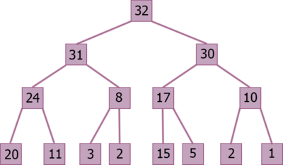
- все узлы в дереве следуют тому свойству, что они больше своих потомков, то есть самый большой элемент находится в корне, и оба его потомка меньше, чем корень, и так далее. Такая куча называется убывающая куча (Max-Heap). Если вместо этого все узлы меньше своих потомков, это называется возрастающая куча (Min-Heap).

Слева на рисунке убывающая куча, справа — возрастающая куча.
Как выстроить дерево
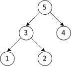
Начиная с идеального бинарного дерева, мы можем изменить его, чтобы оно стало убывающим, запустив функцию heapify для всех неконечных элементов кучи.
Поскольку heapfiy использует рекурсию, это может быть трудно для понимания. Итак, давайте сначала подумаем о том, как бы вы сложили дерево из трех элементов.
heapify(array) Root = array[0] Largest = largest( array[0] , array [2*0 + 1]. array[2*0+2]) if(Root != Largest) Swap(Root, Largest)
В приведенном выше примере показаны два сценария — один, в котором корень является самым большим элементом, и нам не нужно ничего делать. И еще один, в котором корень имеет дочерний элемент большего размера, и нам нужно было поменять их местами, чтобы сохранить свойство убывающей кучи.
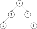
Если вы раньше работали с рекурсивными алгоритмами, то вы поняли, что это должен быть базовый случай.Теперь давайте подумаем о другом сценарии, в котором существует более одного уровня.
На рисунке оба поддерева корневого элемента второго уровня уже являются
убывающими кучами.
Верхний элемент не подходит под убывающую кучу, но все поддеревья являются убывабщими.
Чтобы сохранить свойство убывания для всего дерева, нам нужно будет «протолкнуть» родителя вниз, пока он не достигнет своей правильной позиции.
Таким образом, чтобы сохранить свойство убывания в дереве, где оба поддеревья являются убывающими, нам нужно многократно запускать heapify для корневого элемента, пока он не станет больше, чем его дочерние элементы, или он не станет листовым узлом.
Мы можем объединить оба эти условия в одну функцию heapify следующим образом:
void heapify(int arr[], int n, int i) { int largest = i; int l = 2*i + 1; int r = 2*i + 2; if (l < n && arr[l] > arr[largest]) largest = l; if (right < n && arr[r] > arr[largest]) largest = r; if (largest != i) { swap(arr[i], arr[largest]); // Recursively heapify the affected sub-tree heapify(arr, n, largest); } }Эта функция работает как для базового случая, так и для дерева любого размера. Таким образом, мы можем переместить корневой элемент в правильное положение, чтобы поддерживать статус убывающей кучи для любого размера дерева, пока поддеревья являются убывающими.
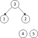
Сборка убывающей кучи
Чтобы собрать убывающую кучу из любого дерева, мы можем начать выстраивать каждое поддерево снизу вверх и получить убывающую кучу после применения функции ко всем элементам, включая корневой элемент.
В случае полного дерева первый индекс неконечного узла определяется как n / 2 — 1. Все остальные узлы после этого являются листовыми узлами и, следовательно, не нуждаются в куче.
Мы можем выстроить убывающую кучу так:
// Build heap (rearrange array) for (int i = n / 2 - 1; i >= 0; i--) heapify(arr, n, i);
Как показано на диаграмме выше, мы начинаем с кучи самых маленьких деревьев и постепенно продвигаемся вверх, пока не достигнем корневого элемента.
Процедуры для Heapsort
- Поскольку дерево удовлетворяет свойству убывающей, самый большой элемент сохраняется в корневом узле.
- Удалите корневой элемент и поместите в конец массива (n-я позиция). Поместите последний элемент дерева (кучу) в свободное место.
- Уменьшите размер кучи на 1 и снова укрупните корневой элемент, чтобы у вас был самый большой элемент в корне.
- Процесс повторяется до тех пор, пока все элементы списка не будут отсортированы.
Код выглядит так:
for (int i=n-1; i>=0; i--) { // Переместить текущий корень в конец swap(arr[0], arr[i]); // вызовите максимальный heapify на уменьшенной куче heapify(arr, i, 0); }Представление
Сортировка кучи имеет O (nlogn) временные сложности для всех случаев (лучший случай, средний случай и худший случай). В чем же причина? Высота полного бинарного дерева, содержащего n элементов, равна log (n).
Как мы видели ранее, чтобы полностью накапливать элемент, чьи поддеревья уже являются убывабщими кучами, нам нужно продолжать сравнивать элемент с его левым и правым потомками и толкать его вниз, пока он не достигнет точки, где оба его потомка меньше его.
В худшем случае нам потребуется переместить элемент из корневого узла в конечный узел, выполнив несколько сравнений и обменов log (n).
На этапе build_max_heap мы делаем это для n / 2 элементов, поэтому сложность шага build_heap в наихудшем случае равна n / 2 * log (n) ~ nlogn.
На этапе сортировки мы обмениваем корневой элемент с последним элементом и подкачиваем корневой элемент. Для каждого элемента это снова занимает большое время, поскольку нам, возможно, придется перенести этот элемент от корня до листа. Поскольку мы повторяем операцию n раз, шаг heap_sort также nlogn.
Кроме того, поскольку шаги build_max_heap и heap_sort выполняются один за другим, алгоритмическая сложность не умножается и остается в порядке nlogn.
Также выполняется сортировка в O (1) пространстве сложности. По сравнению с быстрой сортировкой, в худшем случае (O (nlogn)). Быстрая сортировка имеет сложность O (n ^ 2) для худшего случая. Но в других случаях быстрая сортировка выполняется достаточно быстро. Introsort — это альтернатива heapsort, которая сочетает в себе quicksort и heapsort для сохранения преимуществ, таких как скорость heapsort в худшем случае и средняя скорость quicksort.
Применение сортировки кучей
Системы, связанные с безопасностью, и встроенные системы, такие как ядро Linux, используют сортировку кучей из-за верхней границы O (n log n) времени работы Heapsort и постоянной верхней границы O (1) его вспомогательного хранилища.
Хотя сортировка кучей имеет O (n log n) временную сложность даже для наихудшего случая, у нее нет больше приложений (по сравнению с другими алгоритмами сортировки, такими как быстрая сортировка, сортировка слиянием). Тем не менее, его базовая структура данных, куча, может быть эффективно использована, если мы хотим извлечь наименьший (или наибольший) из списка элементов без дополнительных затрат на сохранение оставшихся элементов в отсортированном порядке. Например, приоритетные очереди.
Реализация сортировки кучи на разных языках программирования
Реализация C ++
// C++ program for implementation of Heap Sort #include <iostream> using namespace std; void heapify(int arr[], int n, int i) { // Find largest among root, left child and right child int largest = i; int l = 2*i + 1; int r = 2*i + 2; if (l < n && arr[l] > arr[largest]) largest = l; if (right < n && arr[r] > arr[largest]) largest = r; // Swap and continue heapifying if root is not largest if (largest != i) { swap(arr[i], arr[largest]); heapify(arr, n, largest); } } // main function to do heap sort void heapSort(int arr[], int n) { // Build max heap for (int i = n / 2 - 1; i >= 0; i--) heapify(arr, n, i); // Heap sort for (int i=n-1; i>=0; i--) { swap(arr[0], arr[i]); // Heapify root element to get highest element at root again heapify(arr, i, 0); } } void printArray(int arr[], int n) { for (int i=0; i<n; ++i) cout << arr[i] << " "; cout << "n"; } int main() { int arr[] = {1,12,9,5,6,10}; int n = sizeof(arr)/sizeof(arr[0]); heapSort(arr, n); cout << "Sorted array is n"; printArray(arr, n); }
Реализация на Java
// Java program for implementation of Heap Sort public class HeapSort { public void sort(int arr[]) { int n = arr.length; // Build max heap for (int i = n / 2 - 1; i >= 0; i--) { heapify(arr, n, i); } // Heap sort for (int i=n-1; i>=0; i--) { int temp = arr[0]; arr[0] = arr[i]; arr[i] = temp; // Heapify root element heapify(arr, i, 0); } } void heapify(int arr[], int n, int i) { // Find largest among root, left child and right child int largest = i; int l = 2*i + 1; int r = 2*i + 2; if (l < n && arr[l] > arr[largest]) largest = l; if (r < n && arr[r] > arr[largest]) largest = r; // Swap and continue heapifying if root is not largest if (largest != i) { int swap = arr[i]; arr[i] = arr[largest]; arr[largest] = swap; heapify(arr, n, largest); } } static void printArray(int arr[]) { int n = arr.length; for (int i=0; i < n; ++i) System.out.print(arr[i]+" "); System.out.println(); } public static void main(String args[]) { int arr[] = {1,12,9,5,6,10}; HeapSort hs = new HeapSort(); hs.sort(arr); System.out.println("Sorted array is"); printArray(arr); } }
Реализация на Python (Python 3)
def heapify(arr, n, i): # Find largest among root and children largest = i l = 2 * i + 1 r = 2 * i + 2 if l < n and arr[i] < arr[l]: largest = l if r < n and arr[largest] < arr[r]: largest = r # If root is not largest, swap with largest and continue heapifying if largest != i: arr[i],arr[largest] = arr[largest],arr[i] heapify(arr, n, largest) def heapSort(arr): n = len(arr) # Build max heap for i in range(n, 0, -1): heapify(arr, n, i) for i in range(n-1, 0, -1): # swap arr[i], arr[0] = arr[0], arr[i] #heapify root element heapify(arr, i, 0) arr = [ 12, 11, 13, 5, 6, 7] heapSort(arr) n = len(arr) print ("Sorted array is") for i in range(n): print ("%d" %arr[i])


Перевод статьи подготовлен специально для студентов курса «Алгоритмы для разработчиков».
Пирамидальная сортировка (или сортировка кучей, HeapSort) — это метод сортировки сравнением, основанный на такой структуре данных как двоичная куча. Она похожа на сортировку выбором, где мы сначала ищем максимальный элемент и помещаем его в конец. Далее мы повторяем ту же операцию для оставшихся элементов.
Что такое двоичная куча?
Давайте сначала определим законченное двоичное дерево. Законченное двоичное дерево — это двоичное дерево, в котором каждый уровень, за исключением, возможно, последнего, имеет полный набор узлов, и все листья расположены как можно левее (Источник Википедия).
Двоичная куча — это законченное двоичное дерево, в котором элементы хранятся в особом порядке: значение в родительском узле больше (или меньше) значений в его двух дочерних узлах. Первый вариант называется max-heap, а второй — min-heap. Куча может быть представлена двоичным деревом или массивом.
Почему для двоичной кучи используется представление на основе массива ?
Поскольку двоичная куча — это законченное двоичное дерево, ее можно легко представить в виде массива, а представление на основе массива является эффективным с точки зрения расхода памяти. Если родительский узел хранится в индексе I, левый дочерний элемент может быть вычислен как 2 I + 1, а правый дочерний элемент — как 2 I + 2 (при условии, что индексирование начинается с 0).
Алгоритм пирамидальной сортировки в порядке по возрастанию:
- Постройте max-heap из входных данных.
- На данном этапе самый большой элемент хранится в корне кучи. Замените его на последний элемент кучи, а затем уменьшите ее размер на 1. Наконец, преобразуйте полученное дерево в max-heap с новым корнем.
- Повторяйте вышеуказанные шаги, пока размер кучи больше 1.
Как построить кучу?
Процедура преобразования в кучу (далее процедура heapify) может быть применена к узлу, только если его дочерние узлы уже преобразованы. Таким образом, преобразование должно выполняться снизу вверх. Давайте разберемся с помощью примера:
Входные данные: 4, 10, 3, 5, 1
         4(0)
        /
     10(1)   3(2)
    /
 5(3)    1(4)
Числа в скобках представляют индексы в представлении данных в виде массива.
Применение процедуры heapify к индексу 1:
         4(0)
        /
    10(1)    3(2)
    /
5(3)    1(4)
Применение процедуры heapify к индексу 0:
        10(0)
        /
     5(1)  3(2)
    /
 4(3)    1(4)
Процедура heapify вызывает себя рекурсивно для создания кучи  сверху вниз.
Рекомендация: Пожалуйста, сначала решите задачу на “PRACTICE”, прежде чем переходить к решению.
C++
// Реализация пирамидальной сортировки на C++
#include <iostream>

using namespace std;

// Процедура для преобразования в двоичную кучу поддерева с корневым узлом i, что является
// индексом в arr[]. n - размер кучи

void heapify(int arr[], int n, int i)
{
    int largest = i;
// Инициализируем наибольший элемент как корень
    int l = 2*i + 1; // левый = 2*i + 1
    int r = 2*i + 2; // правый = 2*i + 2

 // Если левый дочерний элемент больше корня
    if (l < n && arr[l] > arr[largest])
        largest = l;

   // Если правый дочерний элемент больше, чем самый большой элемент на данный момент
    if (r < n && arr[r] > arr[largest])
        largest = r;

    // Если самый большой элемент не корень
    if (largest != i)
    {
        swap(arr[i], arr[largest]);

// Рекурсивно преобразуем в двоичную кучу затронутое поддерево
        heapify(arr, n, largest);
    }
}

// Основная функция, выполняющая пирамидальную сортировку
void heapSort(int arr[], int n)
{
  // Построение кучи (перегруппируем массив)
    for (int i = n / 2 - 1; i >= 0; i--)
        heapify(arr, n, i);

   // Один за другим извлекаем элементы из кучи
    for (int i=n-1; i>=0; i--)
    {
        // Перемещаем текущий корень в конец
        swap(arr[0], arr[i]);

        // вызываем процедуру heapify на уменьшенной куче
        heapify(arr, i, 0);
    }
}

/* Вспомогательная функция для вывода на экран массива размера n*/
void printArray(int arr[], int n)
{
    for (int i=0; i<n; ++i)
        cout << arr[i] << " ";
    cout << "n";
}

// Управляющая программа
int main()
{
    int arr[] = {12, 11, 13, 5, 6, 7};
    int n = sizeof(arr)/sizeof(arr[0]);

    heapSort(arr, n);

    cout << "Sorted array is n";
    printArray(arr, n);
}
Java
// Реализация пирамидальной сортировки на Java
public class HeapSort
{
    public void sort(int arr[])
    {
        int n = arr.length;

        // Построение кучи (перегруппируем массив)
        for (int i = n / 2 - 1; i >= 0; i--)
            heapify(arr, n, i);

        // Один за другим извлекаем элементы из кучи
        for (int i=n-1; i>=0; i--)
        {
            // Перемещаем текущий корень в конец
            int temp = arr[0];
            arr[0] = arr[i];
            arr[i] = temp;

            // Вызываем процедуру heapify на уменьшенной куче
            heapify(arr, i, 0);
        }
    }

    // Процедура для преобразования в двоичную кучу поддерева с корневым узлом i, что является
// индексом в arr[]. n - размер кучи
     void heapify(int arr[], int n, int i)
    {
        int largest = i; // Инициализируем наибольший элемент как корень
        int l = 2*i + 1; // левый = 2*i + 1
        int r = 2*i + 2; // правый = 2*i + 2

           // Если левый дочерний элемент больше корня
        if (l < n && arr[l] > arr[largest])
            largest = l;

          // Если правый дочерний элемент больше, чем самый большой элемент на данный момент
        if (r < n && arr[r] > arr[largest])
            largest = r;
       // Если самый большой элемент не корень
        if (largest != i)
        {
            int swap = arr[i];
            arr[i] = arr[largest];
            arr[largest] = swap;

          // Рекурсивно преобразуем в двоичную кучу затронутое поддерево
            heapify(arr, n, largest);
        }
    }

    /* Вспомогательная функция для вывода на экран массива размера n */
    static void printArray(int arr[])
    {
        int n = arr.length;
        for (int i=0; i<n; ++i)
            System.out.print(arr[i]+" ");
        System.out.println();
    }

    // Управляющая программа
    public static void main(String args[])
    {
        int arr[] = {12, 11, 13, 5, 6, 7};
        int n = arr.length;

        HeapSort ob = new HeapSort();
        ob.sort(arr);

        System.out.println("Sorted array is");
        printArray(arr);
    }
}
Python
# Реализация пирамидальной сортировки на Python

# Процедура для преобразования в двоичную кучу поддерева с корневым узлом i, что является индексом в arr[]. n - размер кучи
def heapify(arr, n, i):
    largest = i # Initialize largest as root
    l = 2 * i + 1   # left = 2*i + 1
    r = 2 * i + 2   # right = 2*i + 2

  # Проверяем существует ли левый дочерний элемент больший, чем корень

    if l < n and arr[i] < arr[l]:
        largest = l

    # Проверяем существует ли правый дочерний элемент больший, чем корень

    if r < n and arr[largest] < arr[r]:
        largest = r

    # Заменяем корень, если нужно
    if largest != i:
        arr[i],arr[largest] = arr[largest],arr[i] # свап

        # Применяем heapify к корню.
        heapify(arr, n, largest)

# Основная функция для сортировки массива заданного размера
def heapSort(arr):
    n = len(arr)

    # Построение max-heap.
    for i in range(n, -1, -1):
        heapify(arr, n, i)

    # Один за другим извлекаем элементы
    for i in range(n-1, 0, -1):
        arr[i], arr[0] = arr[0], arr[i] # свап
        heapify(arr, i, 0)

# Управляющий код для тестирования
arr = [ 12, 11, 13, 5, 6, 7]
heapSort(arr)
n = len(arr)
print ("Sorted array is")
for i in range(n):
    print ("%d" %arr[i]),
# Этот код предоставил Mohit Kumra
C Sharp
// Реализация пирамидальной сортировки на C#
using System;

public class HeapSort
{
    public void sort(int[] arr)
    {
        int n = arr.Length;

        // Построение кучи (перегруппируем массив)
        for (int i = n / 2 - 1; i >= 0; i--)
            heapify(arr, n, i);

       // Один за другим извлекаем элементы из кучи
        for (int i=n-1; i>=0; i--)
        {
            // Перемещаем текущий корень в конец
            int temp = arr[0];
            arr[0] = arr[i];
            arr[i] = temp;

            // вызываем процедуру heapify на уменьшенной куче
            heapify(arr, i, 0);
        }
    }

    // Процедура для преобразования в двоичную кучу поддерева с корневым узлом i, что является
// индексом в arr[]. n - размер кучи

    void heapify(int[] arr, int n, int i)
    {
        int largest = i;
// Инициализируем наибольший элемент как корень
        int l = 2*i + 1; // left = 2*i + 1
        int r = 2*i + 2; // right = 2*i + 2

        // Если левый дочерний элемент больше корня
        if (l < n && arr[l] > arr[largest])
            largest = l;

        // Если правый дочерний элемент больше, чем самый большой элемент на данный момент
        if (r < n && arr[r] > arr[largest])
            largest = r;

        // Если самый большой элемент не корень
        if (largest != i)
        {
            int swap = arr[i];
            arr[i] = arr[largest];
            arr[largest] = swap;

            // Рекурсивно преобразуем в двоичную кучу затронутое поддерево
            heapify(arr, n, largest);
        }
    }

    /* Вспомогательная функция для вывода на экран массива размера n */
    static void printArray(int[] arr)
    {
        int n = arr.Length;
        for (int i=0; i<n; ++i)
            Console.Write(arr[i]+" ");
        Console.Read();
    }

    //Управляющая программа
    public static void Main()
    {
        int[] arr = {12, 11, 13, 5, 6, 7};
        int n = arr.Length;

        HeapSort ob = new HeapSort();
        ob.sort(arr);

        Console.WriteLine("Sorted array is");
        printArray(arr);
    }
}

//Этот код предоставил
// Akanksha Ra (Abby_akku)
PHP
<?php

// Реализация пирамидальной сортировки на Php

// Процедура для преобразования в двоичную кучу поддерева с корневым узлом i, что является
// индексом в arr[]. n - размер кучи

function heapify(&$arr, $n, $i)
{
    $largest = $i; // Инициализируем наибольший элемент как корень
    $l = 2*$i + 1; // левый = 2*i + 1
    $r = 2*$i + 2; // правый = 2*i + 2

    // Если левый дочерний элемент больше корня
    if ($l < $n && $arr[$l] > $arr[$largest])
        $largest = $l;

    //Если правый дочерний элемент больше, чем самый большой элемент на данный момент
    if ($r < $n && $arr[$r] > $arr[$largest])
        $largest = $r;

    // Если самый большой элемент не корень
    if ($largest != $i)
    {
        $swap = $arr[$i];
        $arr[$i] = $arr[$largest];
        $arr[$largest] = $swap;

        // Рекурсивно преобразуем в двоичную кучу затронутое поддерево
        heapify($arr, $n, $largest);
    }
}

//Основная функция, выполняющая пирамидальную сортировку
function heapSort(&$arr, $n)
{
    // Построение кучи (перегруппируем массив)
    for ($i = $n / 2 - 1; $i >= 0; $i--)
        heapify($arr, $n, $i);

    //Один за другим извлекаем элементы из кучи
    for ($i = $n-1; $i >= 0; $i--)
    {
        // Перемещаем текущий корень в конец
        $temp = $arr[0];
            $arr[0] = $arr[$i];
            $arr[$i] = $temp;

        // вызываем процедуру heapify на уменьшенной куче
        heapify($arr, $i, 0);
    }
}

/* Вспомогательная функция для вывода на экран массива размера n */
function printArray(&$arr, $n)
{
    for ($i = 0; $i < $n; ++$i)
        echo ($arr[$i]." ") ;

}

// Управляющая программа
    $arr = array(12, 11, 13, 5, 6, 7);
    $n = sizeof($arr)/sizeof($arr[0]);

    heapSort($arr, $n);

    echo 'Sorted array is ' . "n";

    printArray($arr , $n);

// Этот код предоставил Shivi_Aggarwal
?>
Вывод:
Отсортированный массив:
5 6 7 11 12 13
Здесь предыдущий C-код для справки.
Замечания:
Пирамидальная сортировка — это вполне годный алгоритм. Его типичная реализация не стабильна, но может быть таковой сделана (см. Здесь).
Временная сложность: Временная сложность heapify — O(Logn). Временная сложность createAndBuildHeap() равна O(n), а общее время работы пирамидальной сортировки — O(nLogn).
Применения пирамидальной сортировки:
- Отсортировать почти отсортированный (или отсортированный на K позиций) массив ;
- k самых больших (или самых маленьких) элементов в массиве.
Алгоритм пирамидальной сортировки имеет ограниченное применение, потому что Quicksort (Быстрая сортировка) и Mergesort (Сортировка слиянием) на практике лучше. Тем не менее, сама структура данных кучи используется довольно часто. См. Применения структуры данных кучи
Скриншоты:
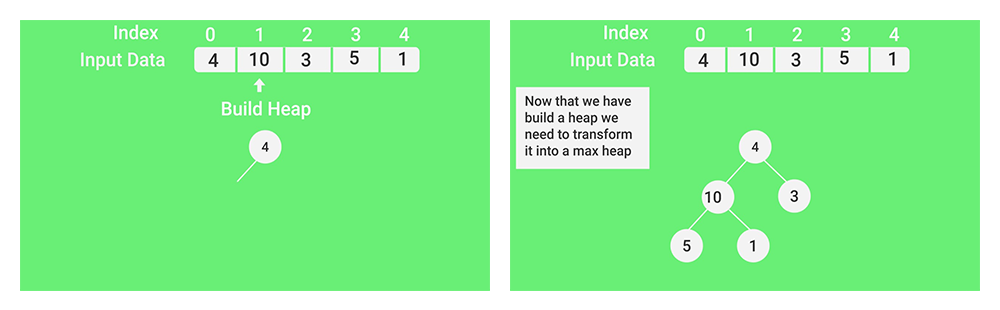
— (Теперь, когда мы построили кучу, мы должны преобразовать ее в max-heap)
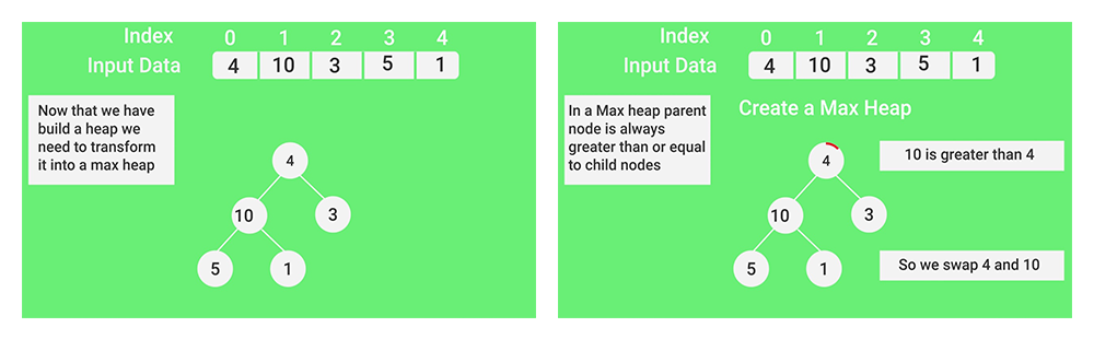
— (В max-heap родительский узел всегда больше или равен по отношению к дочерним
10 больше 4. Поэтому мы меняем местами 4 и 10)
— (В max-heap родительский узел всегда больше или равен по отношению к дочерним
5 больше 4. По этому мы меняем местами 5 и 4)
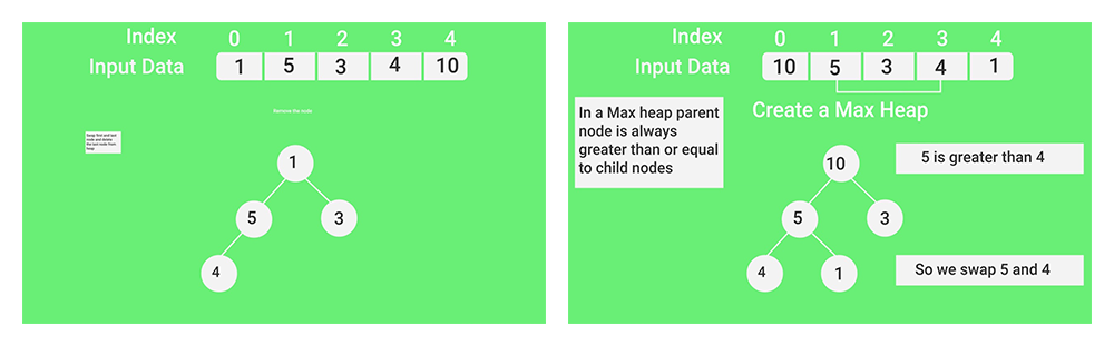
— (Меняем местами первый и последний узлы и удаляем последний из кучи)
Тест по пирамидальной сортировке
Другие алгоритмы сортировки на GeeksforGeeks/GeeksQuiz:
Быстрая сортировка, Сортировка выбором, Сортировка пузырьком, Сортировка вставками, Сортировка слиянием, Пирамидальная сортировка, Поразрядная сортировка, Сортировка подсчетом, Блочная сортировка, Сортировка Шелла, Сортировка расческой, Сортировка подсчетом со списком.
Практикум по сортировке
Пожалуйста, оставляйте комментарии, если вы обнаружите что-то неправильное или вы хотите поделиться дополнительной информацией по обсуждаемой выше теме.
- Подробности
- Категория: Сортировка и поиск
Пирамидальная сортировка (англ. Heapsort, «Сортировка кучей») — алгоритм сортировки, работающий в худшем, в среднем и в лучшем случае (то есть гарантированно) за O(n log n) операций при сортировке n элементов. Количество применяемой служебной памяти не зависит от размера массива (то есть, O(1)).
Может рассматриваться как усовершенствованная сортировка пузырьком, в которой элемент всплывает (min-heap) / тонет (max-heap) по многим путям.
Необходимо отсортировать массив  , размером
  . Построим на базе этого массива за
  невозрастающую кучу. Так как по свойству кучи максимальный элемент находится в корне, то, поменявшись его местами с
 ![A[n - 1]](http://neerc.ifmo.ru/wiki/images/math/f/c/2/fc2868cc76a0d0e7547fbb3face8e9a1.png) , он встанет на свое место. Далее вызовем процедуру
, он встанет на свое место. Далее вызовем процедуру  , предварительно уменьшив
  на
на  . Она за
  просеет
 ![A[0]](http://neerc.ifmo.ru/wiki/images/math/6/5/4/654231fbdf81aaea7e32bc552bf58a0b.png) на нужное место и сформирует новую кучу (так как мы уменьшили ее размер, то куча располагается с по
на нужное место и сформирует новую кучу (так как мы уменьшили ее размер, то куча располагается с по ![A[n - 2]](http://neerc.ifmo.ru/wiki/images/math/5/a/7/5a72863148b487a8c30973b32027eb0f.png) , а элемент
, а элемент ![A[n-1]](http://neerc.ifmo.ru/wiki/images/math/1/7/4/174c5d6c094683ab26f236920cfba0c2.png) находится на своем месте). Повторим эту процедуру для новой кучи, только корень будет менять местами не с , а с
находится на своем месте). Повторим эту процедуру для новой кучи, только корень будет менять местами не с , а с ![A[n-2]](http://neerc.ifmo.ru/wiki/images/math/3/4/d/34d7bc6f3d4794e3e848add044f324c7.png) . Делая аналогичные действия, пока не станет равен , мы будем ставить наибольшее из оставшихся чисел в конец не отсортированной части. Очевидно, что таким образом, мы получим отсортированный массив.
. Делая аналогичные действия, пока не станет равен , мы будем ставить наибольшее из оставшихся чисел в конец не отсортированной части. Очевидно, что таким образом, мы получим отсортированный массив.
| Худшее время |
O(n log n) |
|---|---|
| Лучшее время |
O(n log n) |
| Среднее время |
O(n log n) |
Пусть дана последовательность из  элементов
  .
.
| Массив | Описание шага |
|---|---|
| 5 3 4 1 2 | Строим кучу из исходного массива |
| Первый проход | |
| 2 3 4 1 5 | Меняем местами первый и последний элементы |
| 4 3 2 1 5 | Строим кучу из первых четырех элементов |
| Второй проход | |
| 1 3 2 4 5 | Меняем местами первый и четвертый элементы |
| 3 1 2 4 5 | Строим кучу из первых трех элементов |
| Третий проход | |
| 2 1 3 4 5 | Меняем местами первый и третий элементы |
| 2 1 3 4 5 | Строим кучу из двух элементов |
| Четвертый проход | |
| 1 2 3 4 5 | Меняем местами первый и второй элементы |
| 1 2 3 4 5 | Массив отсортирован |
Реализация алгоритма на различных языках программирования:
C
#include <stdio.h>

#define MAXL 1000

void swap (int *a, int *b)
{
  int t = *a;
  *a = *b;
  *b = t;
}
int main()
{
  int a[MAXL], n, i, sh = 0, b = 0;
  scanf ("%i", &n);
  for (i = 0; i < n; ++i)
    scanf ("%i", &a[i]);
  while (1)
  {
    b = 0;
    for (i = 0; i < n; ++i)
    {
      if (i*2 + 2 + sh < n)
      {
        if (a[i+sh] > a[i*2 + 1 + sh] || a[i + sh] > a[i*2 + 2 + sh])
	{
	  if (a[i*2+1+sh] < a[i*2+2+sh])
	  {
	    swap (&a[i+sh], &a[i*2+1+sh]);
	    b = 1;
	  }
	  else if (a[i*2+2+sh] < a[i*2+1+sh])
	  {
	    swap (&a[i+sh],&a[i*2+2+sh]);
	    b = 1;
	  }
	}
      }
      else if (i * 2 + 1 + sh < n)
      {
        if (a[i+sh] > a[i*2+1+sh])
	{
	  swap (&a[i+sh], &a[i*2+1+sh]);
	  b=1;
	}
      }
    }
    if (!b) sh++;
    if (sh+2==n)
      break;
  }
  for (i = 0; i < n; ++i)
    printf ("%i%c", a[i], (i!=n-1)?' ':'n');
  return 0;
}
C++
#include <iterator>

template< typename Iterator >
void adjust_heap( Iterator first
                  , typename std::iterator_traits< Iterator >::difference_type current
                  , typename std::iterator_traits< Iterator >::difference_type size
                  , typename std::iterator_traits< Iterator >::value_type tmp )
{
    typedef typename std::iterator_traits< Iterator >::difference_type diff_t;

    diff_t top = current, next = 2 * current + 2;

    for ( ; next < size; current = next, next = 2 * next + 2 )
    {
        if ( *(first + next) < *(first + next - 1) )
            --next;
        *(first + current) = *(first + next);
    }

    if ( next == size )
        *(first + current) = *(first + size - 1), current = size - 1;

    for ( next = (current - 1) / 2;
          top > current && *(first + next) < tmp;
          current = next, next = (current - 1) / 2 )
    {
        *(first + current) = *(first + next);
    }
    *(first + current) = tmp;
}

template< typename Iterator >
void pop_heap( Iterator first, Iterator last)
{
    typedef typename std::iterator_traits< Iterator >::value_type value_t;

    value_t tmp = *--last;
    *last = *first;
    adjust_heap( first, 0, last - first, tmp );
}

template< typename Iterator >
void heap_sort( Iterator first, Iterator last )
{
    typedef typename std::iterator_traits< Iterator >::difference_type diff_t;
    for ( diff_t current = (last - first) / 2 - 1; current >= 0; --current )
        adjust_heap( first, current, last - first, *(first + current) );

    while ( first < last )
        pop_heap( first, last-- );
}
C++ (другой вариант)
#include <iostream>
#include <conio.h>

using namespace std;

void iswap(int &n1, int &n2)
{
    int temp = n1;
    n1 = n2;
    n2 = temp;
}

int main()
{
    int const n = 100;
    int a[n];
    for ( int i = 0; i < n; ++i ) { a[i] = n - i; cout << a[i] << " "; }
	//заполняем массив для наглядности.
	//-----------сортировка------------//
	//сортирует по-возрастанию. чтобы настроить по-убыванию,
	//поменяйте знаки сравнения в строчках, помеченных /*(знак)*/
    int sh = 0; //смещение
    bool b = false;
    for(;;)
    {
	b = false;
	for ( int i = 0; i < n; i++ )
	{
	    if( i * 2 + 2 + sh < n )
	    {
		if( ( a[i + sh] > /*<*/ a[i * 2 + 1 + sh] ) || ( a[i + sh] > /*<*/ a[i * 2 + 2 + sh] ) )
		{
		    if ( a[i * 2 + 1 + sh] < /*>*/ a[i * 2 + 2 + sh] )
		    {
			iswap( a[i + sh], a[i * 2 + 1 + sh] );
			b = true;
		    }
		    else if ( a[i * 2 + 2 + sh] < /*>*/ a[ i * 2 + 1 + sh])
		         {
		             iswap( a[ i + sh], a[i * 2 + 2 + sh]);
		             b = true;
		         }
		}
		//дополнительная проверка для последних двух элементов
               //с помощью этой проверки можно отсортировать пирамиду
               //состоящую всего лишь из трех элементов
		    if( a[i*2 + 2 + sh] < /*>*/ a[i*2 + 1 + sh] )
			{
			iswap( a[i*2+1+sh], a[i * 2 +2+ sh] );
                        b = true;
			}
	    }
	    else if( i * 2 + 1 + sh < n )
	         {
	             if( a[i + sh] > /*<*/ a[ i * 2 + 1 + sh] )
	             {
	                 iswap( a[i + sh], a[i * 2 + 1 + sh] );
	                 b = true;
	             }
	         }
	}
	if (!b) sh++; //смещение увеличивается, когда на текущем этапе
		      //сортировать больше нечего
	if ( sh + 2 == n ) break;
    }  //конец сортировки


    cout << endl << endl;
    for ( int i = 0; i < n; ++i ) cout << a[i] << " ";


    getch();
    return 0;
}
C#
static Int32 add2pyramid(Int32[] arr, Int32 i, Int32 N)
        {
            Int32 imax;
            Int32 buf;
            if ((2 * i + 2) < N)
            {
                if (arr[2 * i + 1] < arr[2 * i + 2]) imax = 2 * i + 2;
                else imax = 2 * i + 1;
            }
            else imax = 2 * i + 1;
            if (imax >= N) return i;
            if (arr[i] < arr[imax])
            {
                buf = arr[i];
                arr[i] = arr[imax];
                arr[imax] = buf;
                if (imax < N / 2) i = imax;
            }
            return i;
        }

        static void Pyramid_Sort(Int32[] arr, Int32 len)
        {
            //step 1: building the pyramid
            for (Int32 i = len / 2 - 1; i >= 0; --i)
            {
                long prev_i = i;
                i = add2pyramid(arr, i, len);
                if (prev_i != i) ++i;
            }

            //step 2: sorting
            Int32 buf;
            for (Int32 k = len - 1; k > 0; --k)
            {
                buf = arr[0];
                arr[0] = arr[k];
                arr[k] = buf;
                Int32 i = 0, prev_i = -1;
                while (i != prev_i)
                {
                    prev_i = i;
                    i = add2pyramid(arr, i, k);
                }
            }
        }

        static void Main(string[] args)
        {
              Int32[] arr = new Int32[100];
              //заполняем массив случайными числами
              Random rd = new Random();
              for(Int32 i = 0; i < arr.Length; ++i) {
                 arr[i] = rd.Next(1, 101);
              }
              System.Console.WriteLine("The array before sorting:");
              foreach (Int32 x in arr)
              {
                 System.Console.Write(x + " ");
              }
              //сортировка
              Pyramid_Sort(arr, arr.Length);

              System.Console.WriteLine("nnThe array after sorting:");
              foreach (Int32 x in arr)
              {
                 System.Console.Write(x + " ");
              }
              System.Console.WriteLine("nnPress the <Enter> key");
              System.Console.ReadLine();
        }
C# (другой вариант)
public class Heap<T>
{
	private T[] _array; //массив сортируемых элементов
	private int heapsize;//число необработанных элементов
	private IComparer<T> _comparer;
	public Heap(T[] a, IComparer<T> comparer){
		_array = a;
		heapsize = a.Length;
		_comparer = comparer;
	}

	public void HeapSort(){
		build_max_heap();//Построение пирамиды
		for(int i = _array.Length - 1; i > 0; i--){

			T temp = _array[0];//Переместим текущий максимальный элемент из нулевой позиции в хвост массива
			_array[0] = _array[i];
			_array[i] = temp;

			heapsize--;//Уменьшим число необработанных элементов
			max_heapify(0);//Восстановление свойства пирамиды
		}
	}

	private int parent (int i) { return (i-1)/2; }//Индекс родительского узла
	private int left (int i) { return 2*i+1; }//Индекс левого потомка
	private int right (int i) { return 2*i+2; }//Индекс правого потомка

	//Метод переупорядочивает элементы пирамиды при условии,
        //что элемент с индексом i меньше хотя бы одного из своих потомков, нарушая тем самым свойство невозрастающей пирамиды
	private void max_heapify(int i){
		int l = left(i);
		int r = right(i);
		int lagest = i;
		if (l<heapsize && _comparer.Compare(_array[l], _array[i])>0)
			lagest = l;
		if (r<heapsize && _comparer.Compare(_array[r], _array[lagest])>0)
			lagest = r;
		if (lagest != i)
		{
			T temp = _array[i];
			_array[i] = _array[lagest];
			_array[lagest] = temp;

			max_heapify(lagest);
		}
	}

	//метод строит невозрастающую пирамиду
	private void build_max_heap(){
		int i = (_array.Length-1)/2;

		while(i>=0){
			max_heapify(i);
			i--;
		}
	}

}

public class IntComparer : IComparer<int>
{
	public int Compare(int x, int y) {return x-y;}
}

public static void Main (string[] args)
{
	int[] arr = Console.ReadLine().Split(' ').Select(s=>int.Parse(s)).ToArray();//вводим элементы массива через пробел
	IntComparer myComparer = new IntComparer();//Класс, реализующий сравнение
	Heap<int> heap = new Heap<int>(arr, myComparer);
	heap.HeapSort();
}
Здесь T — любой тип, на множестве элементов которого можно ввести отношение частичного порядка.
Pascal
Вместо «SomeType» следует подставить любой из арифметических типов (например integer).
type  SomeType=integer;
procedure Sort(var Arr: array of SomeType; Count: Integer);

  procedure DownHeap(index, Count: integer; Current: SomeType);
  //Функция пробегает по пирамиде восстанавливая ее
  //Также используется для изначального создания пирамиды
  //Использование: Передать номер следующего элемента в index
  //Процедура пробежит по всем потомкам и найдет нужное место для следующего элемента
  var
    Child: Integer;
  begin
    while index < Count div 2 do begin
      Child := (index+1)*2-1;
      if (Child < Count-1) and (Arr[Child] < Arr[Child+1]) then
        Child:=Child+1;
      if Current >= Arr[Child] then
        break;
      Arr[index] := Arr[Child];
      index := Child;
    end;
    Arr[index] := Current;
  end;

//Основная функция
var
  i: integer;
  Current: SomeType;
begin
  //Собираем пирамиду
  for i := (Count div 2)-1 downto 0 do
    DownHeap(i, Count, Arr[i]);
  //Пирамида собрана. Теперь сортируем
  for i := Count-1 downto 0 do begin
    Current := Arr[i]; //перемещаем верхушку в начало отсортированного списка
    Arr[i] := Arr[0];
    DownHeap(0, i, Current); //находим нужное место в пирамиде для нового элемента
  end;
end;
var tarr:array of SomeType;
i,n:SomeType;
begin
  writeln('Введите размер массива: ');
  readln(n);
  setlength(tarr,n) ;//Выделяем память под динамический массив
  randomize;
  for i:=0 to n-1 do begin
  tarr[i]:=random(500);//Генерируем случайность
  write (tarr[i]:4);
  end;
  writeln();
  writeln('Всё сортирует');
  Sort(tarr,n);
  for i:=0 to n-1 do begin
  write (tarr[i]:4);
  end;
end.
Pascal (другой вариант)
Примечание: myarray = array[1..Size] of integer; N — количество элементов массива
procedure HeapSort(var m: myarray; N: integer);
var
  i: integer;

  procedure Swap(var a,b:integer);
  var
    tmp: integer;
  begin
    tmp:=a;
    a:=b;
    b:=tmp;
  end;

  procedure Sort(Ns: integer);
  var
    i, tmp, pos, mid: integer;
  begin
    mid := Ns div 2;
    for i := mid downto 1 do
    begin
      pos := i;
      while pos<=mid do
      begin
        tmp := pos*2;
        if tmp<Ns then
        begin
          if m[tmp+1]<m[tmp] then
            tmp := tmp+1;
          if m[pos]>m[tmp] then
          begin
            Swap(m[pos], m[tmp]);
            pos := tmp;
          end
          else
            pos := Ns;
        end
        else
          if m[pos]>m[tmp] then
          begin
            Swap(m[pos], m[tmp]);
            pos := Ns;
          end
          else
            pos := Ns;
        end;
      end;
    end;
begin
  for i:=N downto 2 do
  begin
    Sort(i);
    Swap(m[1], m[i]);
  end;
end;
Pascal (третий вариант)
type  TArray=array [1..10] of integer;
//процедура для перессылки записей

procedure swap(var x,y:integer);
var temp:integer;
begin
  temp:=x;
  x:=y;
  y:=temp;
end;

//процедура приведения массива к пирамидальному виду (to pyramide)
procedure toPyr(var data:TArray; n:integer); //n - размерность массива
var i:integer;
begin
  for i:=n div 2 downto 1 do begin
    if 2*i<=n then if data[i]<data[2*i] then swap(data[i],data[2*i]);
    if 2*i+1<=n then if data[i]<data[2*i+1] then swap(data[i],data[2*i+1]);
  end;
end;

//процедура для сдвига массива влево
procedure left(var data:TArray; n:integer);
var i:integer;
    temp:integer;
begin
  temp:=data[1];
  for i:=1 to n-1 do
    data[i]:=data[i+1];
  data[n]:=temp;
end;

//основная программа
var a:TArray;
i,n:integer;
begin
  n:=10;//Не больше 10, потому что массив статический -
        //type  TArray=array [1..10] of integer;
  randomize;
  for i:=1 to n do begin
   a[i]:=random(500);//Генерируем случайность
   write (a[i]:4);
  end;
  for i:=n downto 1 do begin
    topyr(a,i);
    left(a,n);
  end;
  writeln();
  writeln('Сортируем');
  for i:=1 to n do begin
   write (a[i]:4);
   end;
end.
Python
def heapSort(li):
    """Сортирует список в возрастающем порядке с помощью алгоритма пирамидальной сортировки"""

    def downHeap(li, k, n):
        new_elem = li[k]
        while 2*k+1 < n:
            child = 2*k+1
            if child+1 < n and li[child] < li[child+1]:
                child += 1
            if new_elem >= li[child]:
                break
            li[k] = li[child]
            k = child
        li[k] = new_elem

    size = len(li)
    for i in range(size//2-1,-1,-1):
        downHeap(li, i, size)
    for i in range(size-1,0,-1):
        temp = li[i]
        li[i] = li[0]
        li[0] = temp
        downHeap(li, 0, i)
Python (другой вариант)
def heapsort(s):
    sl = len(s)

    def swap(pi, ci):
        if s[pi] < s[ci]:
            s[pi], s[ci] = s[ci], s[pi]

    def sift(pi, unsorted):
        i_gt = lambda a, b: a if s[a] > s[b] else b
        while pi*2+2 < unsorted:
            gtci = i_gt(pi*2+1, pi*2+2)
            swap(pi, gtci)
            pi = gtci
    # heapify
    for i in range((sl/2)-1, -1, -1):
        sift(i, sl)
    # sort
    for i in range(sl-1, 0, -1):
        swap(i, 0)
        sift(0, i)
Perl
@out=(6,4,2,8,5,3,1,6,8,4,3,2,7,9,1)
$N=@out+0;
if($N>1){
    while($sh+2!=$N){
	$b=undef;
	for my$i(0..$N-1){
	    if($i*2+2+$sh<$N){
		if($out[$i+$sh]gt$out[$i*2+1+$sh] || $out[$i+$sh]gt$out[$i*2+2+$sh]){
	            if($out[$i*2+1+$sh]lt$out[$i*2+2+$sh]){
			($out[$i*2+1+$sh],$out[$i+$sh])=($out[$i+$sh],$out[$i*2+1+$sh]);
			$b=1;
		    }elsif($out[$i*2+2+$sh]lt$out[$i*2+1+$sh]){
			($out[$i*2+2+$sh],$out[$i+$sh])=($out[$i+$sh],$out[$i*2+2+$sh]);
			$b=1;
		    }
		}elsif($out[$i*2+2+$sh]lt$out[$i*2+1+$sh]){
		    ($out[$i*2+1+$sh],$out[$i*2+2+$sh])=($out[$i*2+2+$sh],$out[$i*2+1+$sh]);
		    $b=1;
		}
	    }elsif($i*2+1+$sh<$N && $out[$i+$sh]gt$out[$i*2+1+$sh]){
		($out[$i+$sh],$out[$i*2+1+$sh])=($out[$i*2+1+$sh],$out[$i+$sh]);
		$b=1;
	    }
	}
	++$sh if!$b;
	last if$sh+2==$N;
    }
}
Java
/**
 * Класс для сортировки массива целых чисел с помощью кучи.
 * Методы в классе написаны в порядке их использования. Для сортировки
 * вызывается статический метод sort(int[] a)
 */
class HeapSort {
	/**
	 * Размер кучи. Изначально равен размеру сортируемого массива
	 */
	private static int heapSize;

	/**
	 * Сортировка с помощью кучи.
	 * Сначала формируется куча:
	 * @see HeapSort#buildHeap(int[])
	 * Теперь максимальный элемент массива находится в корне кучи. Его нужно
	 * поменять местами с последним элементом и убрать из кучи (уменьшить
	 * размер кучи на 1). Теперь в корне кучи находится элемент, который раньше
	 * был последним в массиве. Нужно переупорядочить кучу так, чтобы
	 * выполнялось основное условие кучи - a[parent]>=a[child]:
	 * @see #heapify(int[], int)
	 * После этого в корне окажется максимальный из оставшихся элементов.
	 * Повторить до тех пор, пока в куче не останется 1 элемент
	 *
	 * @param a сортируемый массив
	 */
	public static void sort(int[] a) {
		buildHeap(a);
		while (heapSize > 1) {
			swap(a, 0, heapSize - 1);
			heapSize--;
			heapify(a, 0);
		}
	}

	/**
	 * Построение кучи. Поскольку элементы с номерами начиная с a.length / 2 + 1
	 * это листья, то нужно переупорядочить поддеревья с корнями в индексах
	 * от 0 до a.length / 2 (метод heapify вызывать в порядке убывания индексов)
	 *
	 * @param a - массив, из которого формируется куча
	 */
	private static void buildHeap(int[] a) {
		heapSize = a.length;
		for (int i = a.length / 2; i >= 0; i--) {
			heapify(a, i);
		}
	}

	/**
	 * Переупорядочивает поддерево кучи начиная с узла i так, чтобы выполнялось
	 * основное свойство кучи - a[parent] >= a[child].
	 *
	 * @param a - массив, из которого сформирована куча
	 * @param i - корень поддерева, для которого происходит переупорядосивание
	 */
	private static void heapify(int[] a, int i) {
		int l = left(i);
		int r = right(i);
		int largest = i;
		if (l < heapSize && a[i] < a[l]) {
			largest = l;
		}
		if (r < heapSize && a[largest] < a[r]) {
			largest = r;
		}
		if (i != largest) {
			swap(a, i, largest);
			heapify(a, largest);
		}
	}

	/**
	 * Возвращает индекс правого потомка текущего узла
	 *
	 * @param i индекс текущего узла кучи
	 * @return индекс правого потомка
	 */
	private static int right(int i) {
		return 2 * i + 1;
	}

	/**
	 * Возвращает индекс левого потомка текущего узла
	 *
	 * @param i индекс текущего узла кучи
	 * @return индекс левого потомка
	 */
	private static int left(int i) {
		return 2 * i + 2;
	}

	/**
	 * Меняет местами два элемента в массиве
	 *
	 * @param a массив
	 * @param i индекс первого элемента
	 * @param j индекс второго элемента
	 */
	private static void swap(int[] a, int i, int j) {
		int temp = a[i];
		a[i] = a[j];
		a[j] = temp;
	}

}
Достоинства
- Имеет доказанную оценку худшего случая
 .
. - Сортирует на месте, то есть требует всего O(1) дополнительной памяти (если дерево организовывать так, как показано выше).
Недостатки
- Сложен в реализации.
- Неустойчив — для обеспечения устойчивости нужно расширять ключ.
- На почти отсортированных массивах работает столь же долго, как и на хаотических данных.
- На одном шаге выборку приходится делать хаотично по всей длине массива — поэтому алгоритм плохо сочетается с кэшированием и подкачкой памяти.
- Методу требуется «мгновенный» прямой доступ; не работает на связанных списках и других структурах памяти последовательного доступа.
Сортировка слиянием при расходе памяти O(n) быстрее ( с меньшей константой) и не подвержена деградации на неудачных данных.
Из-за сложности алгоритма выигрыш получается только на больших n. На небольших n (до нескольких тысяч) быстрее сортировка Шелла.
При написании статьи были использованы открытые источники сети интернет :
Wikipedia
Kvodo
Youtube
Алгоритм пирамидальной сортировки по-английски называется «Heap Sort». «Heap» переводится, как «куча». В связи с этим пирамидальную сортировку ещё называют «сортировка кучей»
Оставим в стороне религиозные споры о преимуществах и недостатках алгоритма Quick Sort, и будем рассматривать пирамидальную сортировку, как самый быстрый алгоритм из доступных (см. Лекцию №3) для сортировки небольших объёмов данных (умещающихся в кеш процессора).
Пирамидальная сортировка была предложена Дж. Уильямсом в 1964 году. Это алгоритм сортировки массива произвольных элементов, не требующий дополнительной памяти и дополнительных структур данных. Время работы алгоритма — $") в среднем, а также в лучшем и худшем случаях.
в среднем, а также в лучшем и худшем случаях.
Везде в этой лекции будем считать, что первый элемент массива имеет индекс 0.
Двоичное дерево
Двоичное дерево — структура данных, в которой каждый элемент имеет левого и/или правого потомка, либо вообще не имеет потомков. В последнем случае элемент называется листовым.
Если элемент A имеет потомка B, то элемент A называется родителем элемента B. В двоичном дереве существует единственный элемент, который не имеет родителей; такой элемент называется корневым.
Пример двоичного дерева показан на рисунке 1:

Рис. 1. Пример двоичного дерева
Почти заполненным двоичным деревом называется двоичное дерево, обладающее тремя свойствами:
- все листовые элементы находятся в нижнем уровне, либо в нижних двух уровнях;
- все листья в уровне заполняют уровень слева;
- все уровни (кроме, быть может, последнего уровня) полностью заполнены элементами.
Дерево на рис. 1 не является почти заполненным, так как уровень 4 не заполнен слева (элемент g «мешает»), и третий уровень (не являющийся последним), не заполнен полностью.
Почти заполненное двоичное дерево можно хранить в массиве без дополнительных затрат. Для этого достаточно перенумеровать элементы каждого уровня слева-направо:

Рис. 2. Пример нумерации элементов почти заполненного дерева
Нетрудно видеть, что при такой нумерации потомки узла с номером n (если есть) имеют номера  и
и  . Родитель узла имеет номер
 /2rightrfloor$") :
:

Рис. 3. Пример нахождения потомков и родителя в массиве
Пирамида
Возрастающей пирамидой называется почти заполненное дерево, в котором значение каждого элемента больше либо равно значения всех его потомков. Аналогично, в убывающей пирамиде значение каждого элемента меньше либо равно значения потомков.
Пример возрастающей пирамиды показан на рисунке:

Рис. 4. Пример возрастающей пирамиды
Очевидно, самое большое значение в возрастающей пирамиде имеет корневой элемент. Однако, из свойств пирамиды не следует, что значения элементов уменьшаются с увеличением уровня. В частности, на рис. 4 элемент со значением 3 на четвёртом уровне больше значений всех элементов, кроме одного, на третьем уровне.
Важной операцией является отделение последнего (в смысле нумерации) элемента от пирамиды. Нетрудно доказать, что в этом случае двоичное дерево остаётся почти заполненным, и все свойства пирамиды сохраняются.
Просеивание вверх
Рассмотрим теперь задачу присоединения элемента с произвольным значением к возрастающей пирамиде. Если просто добавить элемент в конец массива, то свойство пирамиды (значение любого элемента  значения его родителя) может быть нарушено. Для восстановления свойства пирамиды к добавленному элементу применяется процедура просеивания вверх, которая описывается следующим алгоритмом:
- если элемент корневой, или его значение значения родителя, то конец;
- меняем местами значения элемента и его родителя;
- выполняем процедуру просеивания вверх для родителя.
После выполнения данной процедуры свойство пирамиды будет восстановлено, так как:
- Если вновь добавленный элемент больше родителя, то он больше и второго потомка родителя, так как до добавления нового элемента было выполнено свойство пирамиды, и родитель был не меньше своего потомка. Поэтому после обмена значений элемента и родителя свойство пирамиды будет восстановлено в поддереве, корнем которого является родитель с новым значением.
- Но свойство пирамиды может быть нарушено в отношении родителя и родителя родителя (так как значение родителя стало больше). Процедура вызывается для родительского узла, чтобы восстановить это свойство.
Исходный код процедуры просеивания вверх я не привожу, так как он нам не понадобится. Пример просеивания вверх показан на рисунке:

Рис. 5. Процесс просеивания вверх добавленного элемента
Просеивание вниз
Что делать, если нам нужно заменить корневой элемент на какой-либо другой? В этом случае пирамидальную структуру двоичного дерева можно восстановить с помощью процедуры просеивания вниз:
- если элемент листовой, или его значение значений потомков, то конец;
- меняем местами значения элемента и его потомка, имеющего максимальное значение;
- выполняем процедуру просеивания вниз для изменившегося потомка.
 значений потомков, то конец;
Исходный код процедуры просеивания вниз приведён в листинге 1:
template<class T> void SiftDown(T* const heap,int i,int const n)
{ //Просеивает элемент номер i вниз в пирамиде heap.
//n — размер пирамиды
//Идея в том, что вычисляется максимальный элемент из трёх:
// 1) текущий элемент
// 2) левый потомок
// 3) правый потомок
//Если индекс текущего элемента не равен индексу максималь-
// ного, то меняю их местами, и перехожу к максимальному
//Индекс максимального элемента с «предыдущей» итерации:
int nMax( i );
//Значение текущего элемента (не меняется):
T const value( heap[i] );
while(true)
{
//Номер текущего элемента — это номер максимального
// элемента с предыдущей итерации:
i = nMax;
int childN( i*2+1 ); //Индекс левого потомка
//Если есть левый потомок и он больше текущего элемента,
if ( ( childN < n ) && ( heap[childN] > value ) )
nMax = childN; // то он становится максимальным
++childN; //Индекс правого потомка
//Если есть правый потомок и он больше максимального,
if ( ( childN < n ) && ( heap[childN] > heap[nMax] ) )
nMax = childN; // то он становится максимальным
//Текущий элемент является максимальным —
// конец просеивания:
if (nMax == i) break;
//Меняю местами текущий элемент с максимальным:
heap[i] = heap[nMax]; heap[nMax] = value;
// при этом значение value будет в ячейке nMax,
// поэтому в начале следующей итерации значение value
// правильно, т.к. мы переходим именно к этой ячейке
};
}
Листинг 1. Функция просеивания вниз в возрастающей пирамиде
Пример просеивания вниз показан на рисунке:

Рис. 6. Процесс просеивания вниз изменённого корневого элемента
Построение пирамиды
Допустим, у нас есть произвольный набор из n элементов, и мы хотим построить из него пирамиду. Самый простой способ этого добиться — начать с пустой пирамиды, и добавлять в неё элементы один за другим, каждый раз вызывая процедуру просеивания вверх для нового элемента. Назовём этот метод построения пирамиды «методом просеивания вверх». Пример работы алгоритма показан на рисунке:

Рис. 7. Анимация простого алгоритма построения пирамиды
Рассчитаем быстродействие этого метода в самом плохом случае. Пусть массив уже отсортирован по возрастанию, и каждый добавляемый элемент вынужден просеиваться вверх до самого корня. Тогда при добавлении элемента номер i нам потребуется right)$") операций. Мы делаем эту процедуру для всех i от 0 до
операций. Мы делаем эту процедуру для всех i от 0 до  :
:
=sum_{i=0}^{n-1}{Oleft(lnleft(i+1right)right)}=Oleft(sum_{i=1}^n{ln i}right).$$") |
(1) |
Оценим сумму в выражении (1) с помощью определённого интеграла:
dx}<sum_{i=1}^n{ln i}<intlimits_2^{n+1}{ln xdx}.$$") |
(2) |
Вычисляя интегралы, получаем:
cdotlnleft(n+1right)-n-2ln2+1.$$") |
(3) |
Это означает, что:
=Oleft(ncdotln nright).$$") |
(4) |
На самом деле пирамиду можно построить быстрее. Для этого заполним дерево элементами в случайном порядке (например так, как они идут в массиве изначально), и будем его исправлять.
Заметим, что если у нас есть две пирамиды, то, если их соединить общим корнем, а затем просеять корень вниз, то мы получим новую большую пирамиду. Деревья, состоящие из одного элемента, заведомо являются пирамидами, поэтому начнём с набора листовых элементов, а затем будем соединять имеющиеся пирамиды попарно до тех пор, пока не получим одну большую пирамиду. Первый добавляемый корень имеет индекс  . Алгоритм следующий: «для всех i от
  до 0 вызываем процедуру просеивания элемента вниз». Назовём этот метод построения пирамиды «методом просеивания вниз».
Вычислим быстродействие этого алгоритма в худшем случае. Пусть массив отсортирован по возрастанию, и каждый добавляемый корень должен быть просеян в самый низ. Высота дерева примерно равна  , глубина залегания элемента номер i в дереве равна
  , поэтому он будет просеиваться вниз
  шагов. Тогда общее время построения пирамиды будет равно:
=Oleft(sum_{i=n/2}^1{left(ln n-ln iright)}right).$$") |
(5) |
Оценивая сумму интегралами аналогично (2), (3), получим:
=Oleft(nright).$$") |
(6) |
В дальнейшем будем строить пирамиду методом просеивания вниз.
Сортировка
Имея построенную пирамиду, несложно реализовать сортировку. Так как корневой узел пирамиды имеет самое большое значение, мы можем отделить его и поместить в конец массива. Вместо корневого узла можно поставить последний узел дерева и, просеяв его вниз, снова получить пирамиду. В новом дереве корень имеет самое большое значение среди оставшихся элементов. Его снова можно отделить, и так далее. Алгоритм получается следующий:
- поменять местами значения первого и последнего узлов пирамиды;
- отделить последний узел от дерева, уменьшив размер дерева на единицу (элемент остаётся в массиве);
- восстановить пирамиду, просеяв вниз её новый корневой элемент;
- перейти к пункту 1;
По мере работы алгоритма, часть массива, занятая деревом, уменьшается, а в конце массива накапливается отсортированный результат.
Реализация пирамидальной сортировки на языке программирования C++ приведена в листинге 2 (используется процедура просеивания вниз из листинга 1):
template<class T> void HeapSort(T* const heap, int n)
{ //Пирамидальная сортировка массива heap.
// n — размер массива
//Этап 1: построение пирамиды из массива
for(int i(n/2—1); i>=0; —i) SiftDown(heap, i, n);
//Этап 2: сортировка с помощью пирамиды.
// Здесь под «n» понимается размер пирамиды
while( n > 1 ) //Пока в пирамиде больше одного элемента
{
—n; //Отделяю последний элемент
//Меняю местами корневой элемент и отделённый:
T const firstElem( heap[0] );
heap[0] = heap[n];
heap[n] = firstElem;
//Просеиваю новый корневой элемент:
SiftDown(heap, 0, n);
}
}
Листинг 2. Пирамидальная сортировка
Теоретическое время работы этого алгоритма нетрудно оценить, если заметить, что пирамидальная сортировка (без учёта начального построения пирамиды) полностью аналогична построению пирамиды методом просеивания вверх, только производится «в обратном порядке»: пирамида не строится, а «разбирается» элемент-за-элементом, и элементы просеиваются не вверх, а вниз. Поэтому время работы алгоритма пирамидальной сортировки  без учёта времени построения пирамиды будет определяться аналогично формуле (4):
=Oleft(ncdotln nright).$$") |
(7) |
Тогда общее время сортировки (с учётом построения пирамиды) будет равно:
=T_2left(nright)+T_3left(nright)=Oleft(nright)+Oleft(ncdotln nright)=Oleft(ncdotln nright).$$") |
(8) |
Измерение быстродействия алгоритма
Мы уже выяснили с помощью теоретических оценок, что время работы алгоритма пирамидальной сортировки равно: =Oleft(ncdotlnleft(nright)right)$") . Полезно также знать, чему равен неизвестный коэффициент перед
. Полезно также знать, чему равен неизвестный коэффициент перед $") при выполнении сортировки на реальной вычислительной системе.
при выполнении сортировки на реальной вычислительной системе.
На рис. 8 показан график величины $") , определяемой выражением:
, определяемой выражением:
=10^9cdotfrac{Tleft(nright)}{ncdotlnleft(n+1right)},$$") |
(9) |
где n — количество сортируемых псевдослучайных четырёхбайтовых целых чисел, $") — время сортировки на моём компьютере.
— время сортировки на моём компьютере.
Мой процессор: Intel Mobile Core 2 Duo T7500 (во время тестов программа работала на одном ядре). Тактовая частота: 2.2 ГГц. Кэш L2: 4 МБ, 16-ассоциативный, 64 байта на строку.
Для каждого числа элементов было выполнено восемь тестов, и из их результатов был взят минимум, чтобы исключить случайное влияние других вычислительных задач на ход эксперимента.

Рис. 8. Отношение времени пирамидальной сортировки к $")
На графике проявляются две важные особенности алгоритма:
- Алгоритм относительно медленно работает, когда число сортируемых элементов меньше сотни. Для малого числа элементов желательно использовать сортировочные сети; об этом я расскажу в одной из следующих лекций.
- Когда количество сортируемых данных начинает превышать размер кэша (в нашем случае миллион чисел по 4 байта), скорость сортировки падает. Это вызвано тем, что алгоритм обращается к элементам массива довольно случайным образом (с точки зрения алгоритма работы кеша). По мере того, как всё меньшая часть данных уменьшается в кеше, скорость работы алгоритма всё более определяется скоростью работы оперативной памяти, а не скоростью работы кеша. В одной из следующих лекций мы устраним этот недостаток.
Heap Sort is a popular and efficient sorting algorithm in computer programming. Learning how to write the heap sort algorithm requires knowledge of two types of data structures — arrays and trees.
The initial set of numbers that we want to sort is stored in an array e.g. [10, 3, 76, 34, 23, 32] and after sorting, we get a sorted array [3,10,23,32,34,76].
Heap sort works by visualizing the elements of the array as a special kind of complete binary tree called a heap.
Note: As a prerequisite, you must know about a complete binary tree and heap data structure.
Relationship between Array Indexes and Tree Elements
A complete binary tree has an interesting property that we can use to find the children and parents of any node.
If the index of any element in the array is i, the element in the index 2i+1 will become the left child and element in 2i+2 index will become the right child. Also, the parent of any element at index i is given by the lower bound of (i-1)/2.

Let’s test it out,
Left child of 1 (index 0)
= element in (2*0+1) index
= element in 1 index
= 12


Right child of 1
= element in (2*0+2) index
= element in 2 index
= 9

Similarly,
Left child of 12 (index 1)
= element in (2*1+1) index
= element in 3 index
= 5

Right child of 12
= element in (2*1+2) index
= element in 4 index
= 6
Let us also confirm that the rules hold for finding parent of any node
Parent of 9 (position 2)
= (2-1)/2
= ½
= 0.5
~ 0 index
= 1

Parent of 12 (position 1)
= (1-1)/2
= 0 index
= 1
Understanding this mapping of array indexes to tree positions is critical to understanding how the Heap Data Structure works and how it is used to implement Heap Sort.
What is Heap Data Structure?
Heap is a special tree-based data structure. A binary tree is said to follow a heap data structure if
- it is a complete binary tree
- All nodes in the tree follow the property that they are greater than their children i.e. the largest element is at the root and both its children and smaller than the root and so on. Such a heap is called a max-heap. If instead, all nodes are smaller than their children, it is called a min-heap
The following example diagram shows Max-Heap and Min-Heap.

To learn more about it, please visit Heap Data Structure.
How to «heapify» a tree
Starting from a complete binary tree, we can modify it to become a Max-Heap by running a function called heapify on all the non-leaf elements of the heap.
Since heapify uses recursion, it can be difficult to grasp. So let’s first think about how you would heapify a tree with just three elements.
heapify(array)
    Root = array[0]
    Largest = largest( array[0] , array [2*0 + 1]. array[2*0+2])
    if(Root != Largest)
          Swap(Root, Largest)
The example above shows two scenarios — one in which the root is the largest element and we don’t need to do anything. And another in which the root had a larger element as a child and we needed to swap to maintain max-heap property.
If you’re worked with recursive algorithms before, you’ve probably identified that this must be the base case.
Now let’s think of another scenario in which there is more than one level.

The top element isn’t a max-heap but all the sub-trees are max-heaps.
To maintain the max-heap property for the entire tree, we will have to keep pushing 2 downwards until it reaches its correct position.

Thus, to maintain the max-heap property in a tree where both sub-trees are max-heaps, we need to run heapify on the root element repeatedly until it is larger than its children or it becomes a leaf node.
We can combine both these conditions in one heapify function as
void heapify(int arr[], int n, int i) {
  // Find largest among root, left child and right child
  int largest = i;
  int left = 2 * i + 1;
  int right = 2 * i + 2;

  if (left < n && arr[left] > arr[largest])
    largest = left;

  if (right < n && arr[right] > arr[largest])
    largest = right;

    // Swap and continue heapifying if root is not largest
    if (largest != i) {
      swap(&arr[i], &arr[largest]);
      heapify(arr, n, largest);
  }
}
This function works for both the base case and for a tree of any size. We can thus move the root element to the correct position to maintain the max-heap status for any tree size as long as the sub-trees are max-heaps.
Build max-heap
To build a max-heap from any tree, we can thus start heapifying each sub-tree from the bottom up and end up with a max-heap after the function is applied to all the elements including the root element.
In the case of a complete tree, the first index of a non-leaf node is given by n/2 - 1. All other nodes after that are leaf-nodes and thus don’t need to be heapified.
So, we can build a maximum heap as
    // Build heap (rearrange array)
    for (int i = n / 2 - 1; i >= 0; i--)
      heapify(arr, n, i);


As shown in the above diagram, we start by heapifying the lowest smallest trees and gradually move up until we reach the root element.
If you’ve understood everything till here, congratulations, you are on your way to mastering the Heap sort.
Working of Heap Sort
- Since the tree satisfies Max-Heap property, then the largest item is stored at the root node.
- Swap: Remove the root element and put at the end of the array (nth position) Put the last item of the tree (heap) at the vacant place.
- Remove: Reduce the size of the heap by 1.
- Heapify: Heapify the root element again so that we have the highest element at root.
- The process is repeated until all the items of the list are sorted.

The code below shows the operation.
    // Heap sort
    for (int i = n - 1; i >= 0; i--) {
      swap(&arr[0], &arr[i]);

      // Heapify root element to get highest element at root again
      heapify(arr, i, 0);
    }
# Heap Sort in python
def heapify(arr, n, i):
# Find largest among root and children
largest = i
l = 2 * i + 1
r = 2 * i + 2
if l < n and arr[i] < arr[l]:
largest = l
if r < n and arr[largest] < arr[r]:
largest = r
# If root is not largest, swap with largest and continue heapifying
if largest != i:
arr[i], arr[largest] = arr[largest], arr[i]
heapify(arr, n, largest)
def heapSort(arr):
n = len(arr)
# Build max heap
for i in range(n//2, -1, -1):
heapify(arr, n, i)
for i in range(n-1, 0, -1):
# Swap
arr[i], arr[0] = arr[0], arr[i]
# Heapify root element
heapify(arr, i, 0)
arr = [1, 12, 9, 5, 6, 10]
heapSort(arr)
n = len(arr)
print("Sorted array is")
for i in range(n):
print("%d " % arr[i], end='')
// Heap Sort in Java

  public class HeapSort {

    public void sort(int arr[]) {
      int n = arr.length;

      // Build max heap
      for (int i = n / 2 - 1; i >= 0; i--) {
        heapify(arr, n, i);
      }

      // Heap sort
      for (int i = n - 1; i >= 0; i--) {
        int temp = arr[0];
        arr[0] = arr[i];
        arr[i] = temp;

        // Heapify root element
        heapify(arr, i, 0);
      }
    }

    void heapify(int arr[], int n, int i) {
      // Find largest among root, left child and right child
      int largest = i;
      int l = 2 * i + 1;
      int r = 2 * i + 2;

      if (l < n && arr[l] > arr[largest])
        largest = l;

      if (r < n && arr[r] > arr[largest])
        largest = r;

      // Swap and continue heapifying if root is not largest
      if (largest != i) {
        int swap = arr[i];
        arr[i] = arr[largest];
        arr[largest] = swap;

        heapify(arr, n, largest);
      }
    }

    // Function to print an array
    static void printArray(int arr[]) {
      int n = arr.length;
      for (int i = 0; i < n; ++i)
        System.out.print(arr[i] + " ");
      System.out.println();
    }

    // Driver code
    public static void main(String args[]) {
      int arr[] = { 1, 12, 9, 5, 6, 10 };

      HeapSort hs = new HeapSort();
      hs.sort(arr);

      System.out.println("Sorted array is");
      printArray(arr);
    }
  }
// Heap Sort in C
#include <stdio.h>
// Function to swap the the position of two elements
void swap(int *a, int *b) {
int temp = *a;
*a = *b;
*b = temp;
}
void heapify(int arr[], int n, int i) {
// Find largest among root, left child and right child
int largest = i;
int left = 2 * i + 1;
int right = 2 * i + 2;
if (left < n && arr[left] > arr[largest])
largest = left;
if (right < n && arr[right] > arr[largest])
largest = right;
// Swap and continue heapifying if root is not largest
if (largest != i) {
swap(&arr[i], &arr[largest]);
heapify(arr, n, largest);
}
}
// Main function to do heap sort
void heapSort(int arr[], int n) {
// Build max heap
for (int i = n / 2 - 1; i >= 0; i--)
heapify(arr, n, i);
// Heap sort
for (int i = n - 1; i >= 0; i--) {
swap(&arr[0], &arr[i]);
// Heapify root element to get highest element at root again
heapify(arr, i, 0);
}
}
// Print an array
void printArray(int arr[], int n) {
for (int i = 0; i < n; ++i)
printf("%d ", arr[i]);
printf("n");
}
// Driver code
int main() {
int arr[] = {1, 12, 9, 5, 6, 10};
int n = sizeof(arr) / sizeof(arr[0]);
heapSort(arr, n);
printf("Sorted array is n");
printArray(arr, n);
}// Heap Sort in C++
#include <iostream>
using namespace std;
void heapify(int arr[], int n, int i) {
// Find largest among root, left child and right child
int largest = i;
int left = 2 * i + 1;
int right = 2 * i + 2;
if (left < n && arr[left] > arr[largest])
largest = left;
if (right < n && arr[right] > arr[largest])
largest = right;
// Swap and continue heapifying if root is not largest
if (largest != i) {
swap(arr[i], arr[largest]);
heapify(arr, n, largest);
}
}
// main function to do heap sort
void heapSort(int arr[], int n) {
// Build max heap
for (int i = n / 2 - 1; i >= 0; i--)
heapify(arr, n, i);
// Heap sort
for (int i = n - 1; i >= 0; i--) {
swap(arr[0], arr[i]);
// Heapify root element to get highest element at root again
heapify(arr, i, 0);
}
}
// Print an array
void printArray(int arr[], int n) {
for (int i = 0; i < n; ++i)
cout << arr[i] << " ";
cout << "n";
}
// Driver code
int main() {
int arr[] = {1, 12, 9, 5, 6, 10};
int n = sizeof(arr) / sizeof(arr[0]);
heapSort(arr, n);
cout << "Sorted array is n";
printArray(arr, n);
}Heap Sort Complexity
| Time Complexity | |
|---|---|
| Best | O(nlog n) |
| Worst | O(nlog n) |
| Average | O(nlog n) |
| Space Complexity | O(1) |
| Stability | No |
Heap Sort has O(nlog n) time complexities for all the cases ( best case, average case, and worst case).
Let us understand the reason why. The height of a complete binary tree containing n elements is log n
As we have seen earlier, to fully heapify an element whose subtrees are already max-heaps, we need to keep comparing the element with its left and right children and pushing it downwards until it reaches a point where both its children are smaller than it.
In the worst case scenario, we will need to move an element from the root to the leaf node making a multiple of log(n) comparisons and swaps.
During the build_max_heap stage, we do that for n/2 elements so the worst case complexity of the build_heap step is n/2*log n ~ nlog n.
During the sorting step, we exchange the root element with the last element and heapify the root element. For each element, this again takes log n worst time because we might have to bring the element all the way from the root to the leaf. Since we repeat this n times, the heap_sort step is also nlog n.
Also since the build_max_heap and heap_sort steps are executed one after another, the algorithmic complexity is not multiplied and it remains in the order of nlog n.
Also it performs sorting in O(1) space complexity. Compared with Quick Sort, it has a better worst case ( O(nlog n) ). Quick Sort has complexity O(n^2) for worst case. But in other cases, Quick Sort is fast. Introsort is an alternative to heapsort that combines quicksort and heapsort to retain advantages of both: worst case speed of heapsort and average speed of quicksort.
Heap Sort Applications
Systems concerned with security and embedded systems such as Linux Kernel use Heap Sort because of the O(n log n) upper bound on Heapsort’s running time and constant O(1) upper bound on its auxiliary storage.
Although Heap Sort has O(n log n) time complexity even for the worst case, it doesn’t have more applications ( compared to other sorting algorithms like Quick Sort, Merge Sort ). However, its underlying data structure, heap, can be efficiently used if we want to extract the smallest (or largest) from the list of items without the overhead of keeping the remaining items in the sorted order. For e.g Priority Queues.
Similar Sorting Algorithms
- Quicksort
- Merge Sort
A run of heapsort sorting an array of randomly permuted values. In the first stage of the algorithm the array elements are reordered to satisfy the heap property. Before the actual sorting takes place, the heap tree structure is shown briefly for illustration. |
|
| Class | Sorting algorithm |
|---|---|
| Data structure | Array |
| Worst-case performance |  |
| Best-case performance | (distinct keys) or  (equal keys) (equal keys) |
| Average performance | |
| Worst-case space complexity | total  auxiliary auxiliary |
In computer science, heapsort is a comparison-based sorting algorithm. Heapsort can be thought of as an improved selection sort: like selection sort, heapsort divides its input into a sorted and an unsorted region, and it iteratively shrinks the unsorted region by extracting the largest element from it and inserting it into the sorted region. Unlike selection sort, heapsort does not waste time with a linear-time scan of the unsorted region; rather, heap sort maintains the unsorted region in a heap data structure to more quickly find the largest element in each step.[1]
Although somewhat slower in practice on most machines than a well-implemented quicksort, it has the advantage of a more favorable worst-case O(n log n) runtime (and as such is used by Introsort as a fallback should it detect that quicksort is becoming degenerate). Heapsort is an in-place algorithm, but it is not a stable sort.
Heapsort was invented by J. W. J. Williams in 1964.[2] This was also the birth of the heap, presented already by Williams as a useful data structure in its own right.[3] In the same year, Robert W. Floyd published an improved version that could sort an array in-place, continuing his earlier research into the treesort algorithm.[3]
Overview[edit]
The heapsort algorithm can be divided into two parts.
In the first step, a heap is built out of the data (see Binary heap § Building a heap). The heap is often placed in an array with the layout of a complete binary tree. The complete binary tree maps the binary tree structure into the array indices; each array index represents a node; the index of the node’s parent, left child branch, or right child branch are simple expressions. For a zero-based array, the root node is stored at index 0; if i is the index of the current node, then
  iParent(i)     = floor((i-1) / 2) where floor functions map a real number to the largest leading integer.
  iLeftChild(i)  = 2*i + 1
  iRightChild(i) = 2*i + 2
In the second step, a sorted array is created by repeatedly removing the largest element from the heap (the root of the heap), and inserting it into the array. The heap is updated after each removal to maintain the heap property. Once all objects have been removed from the heap, the result is a sorted array.
Heapsort can be performed in place. The array can be split into two parts, the sorted array and the heap. The storage of heaps as arrays is diagrammed here. The heap’s invariant is preserved after each extraction, so the only cost is that of extraction.
Algorithm[edit]
The heapsort algorithm involves preparing the list by first turning it into a max heap. The algorithm then repeatedly swaps the first value of the list with the last value, decreasing the range of values considered in the heap operation by one, and sifting the new first value into its position in the heap. This repeats until the range of considered values is one value in length.
The steps are:
- Call the
buildMaxHeap()function on the list. Also referred to asheapify(), this builds a heap from a list in operations. - Swap the first element of the list with the final element. Decrease the considered range of the list by one.
- Call the
siftDown()function on the list to sift the new first element to its appropriate index in the heap. - Go to step (2) unless the considered range of the list is one element.
The buildMaxHeap() operation is run once, and is O(n) in performance. The siftDown() function is O(log n), and is called n times. Therefore, the performance of this algorithm is O(n + n log n) = O(n log n).
Pseudocode[edit]
The following is a simple way to implement the algorithm in pseudocode. Arrays are zero-based and swap is used to exchange two elements of the array. Movement ‘down’ means from the root towards the leaves, or from lower indices to higher. Note that during the sort, the largest element is at the root of the heap at a[0], while at the end of the sort, the largest element is in a[end].
procedure heapsort(a, count) is
    input: an unordered array a of length count

    (Build the heap in array a so that largest value is at the root)
    heapify(a, count)

    (The following loop maintains the invariants that a[0:end] is a heap and every element
     beyond end is greater than everything before it (so a[end:count] is in sorted order))
    end ← count - 1
    while end > 0 do
        (a[0] is the root and largest value. The swap moves it in front of the sorted elements.)
        swap(a[end], a[0])
        (the heap size is reduced by one)
        end ← end - 1
        (the swap ruined the heap property, so restore it)
        siftDown(a, 0, end)
The sorting routine uses two subroutines, heapify and siftDown. The former is the common in-place heap construction routine, while the latter is a common subroutine for implementing heapify.
(Put elements of 'a' in heap order, in-place)
procedure heapify(a, count) is
    (start is assigned the index in 'a' of the last parent node)
    (the last element in a 0-based array is at index count-1; find the parent of that element)
    start ← iParent(count-1)

    while start ≥ 0 do
        (sift down the node at index 'start' to the proper place such that all nodes below
         the start index are in heap order)
        siftDown(a, start, count - 1)
        (go to the next parent node)
        start ← start - 1
    (after sifting down the root all nodes/elements are in heap order)

(Repair the heap whose root element is at index 'start', assuming the heaps rooted at its children are valid)
procedure siftDown(a, start, end) is
    root ← start

    while iLeftChild(root) ≤ end do    (While the root has at least one child)
        child ← iLeftChild(root)   (Left child of root)
        swap ← root                (Keeps track of child to swap with)

        if a[swap] < a[child] then
            swap ← child
        (If there is a right child and that child is greater)
        if child+1 ≤ end and a[swap] < a[child+1] then
            swap ← child + 1
        if swap = root then
            (The root holds the largest element. Since we assume the heaps rooted at the
             children are valid, this means that we are done.)
            return
        else
            Swap(a[root], a[swap])
            root ← swap          (repeat to continue sifting down the child now)
The heapify procedure can be thought of as building a heap from the bottom up by successively sifting downward to establish the heap property. An alternative version (shown below) that builds the heap top-down and sifts upward may be simpler to understand. This siftUp version can be visualized as starting with an empty heap and successively inserting elements, whereas the siftDown version given above treats the entire input array as a full but «broken» heap and «repairs» it starting from the last non-trivial sub-heap (that is, the last parent node).

Difference in time complexity between the «siftDown» version and the «siftUp» version.
Also, the siftDown version of heapify has O(n) time complexity, while the siftUp version given below has O(n log n) time complexity due to its equivalence with inserting each element, one at a time, into an empty heap.[4]
This may seem counter-intuitive since, at a glance, it is apparent that the former only makes half as many calls to its logarithmic-time sifting function as the latter; i.e., they seem to differ only by a constant factor, which never affects asymptotic analysis.
To grasp the intuition behind this difference in complexity, note that the number of swaps that may occur during any one siftUp call increases with the depth of the node on which the call is made. The crux is that there are many (exponentially many) more «deep» nodes than there are «shallow» nodes in a heap, so that siftUp may have its full logarithmic running-time on the approximately linear number of calls made on the nodes at or near the «bottom» of the heap. On the other hand, the number of swaps that may occur during any one siftDown call decreases as the depth of the node on which the call is made increases. Thus, when the siftDown heapify begins and is calling siftDown on the bottom and most numerous node-layers, each sifting call will incur, at most, a number of swaps equal to the «height» (from the bottom of the heap) of the node on which the sifting call is made. In other words, about half the calls to siftDown will have at most only one swap, then about a quarter of the calls will have at most two swaps, etc.
The heapsort algorithm itself has O(n log n) time complexity using either version of heapify.
 procedure heapify(a,count) is
     (end is assigned the index of the first (left) child of the root)
     end := 1

     while end < count
         (sift up the node at index end to the proper place such that all nodes above
          the end index are in heap order)
         siftUp(a, 0, end)
         end := end + 1
     (after sifting up the last node all nodes are in heap order)

 procedure siftUp(a, start, end) is
     input:  start represents the limit of how far up the heap to sift.
                   end is the node to sift up.
     child := end
     while child > start
         parent := iParent(child)
         if a[parent] < a[child] then (out of max-heap order)
             swap(a[parent], a[child])
             child := parent (repeat to continue sifting up the parent now)
         else
             return
Note that unlike siftDown approach where, after each swap, you need to call only the siftDown subroutine to fix the broken heap; the siftUp subroutine alone cannot fix the broken heap. The heap needs to be built every time after a swap by calling the heapify procedure since «siftUp» assumes that the element getting swapped ends up in its final place, as opposed to «siftDown» allows for continuous adjustments of items lower in the heap until the invariant is satisfied. The adjusted pseudocode for using siftUp approach is given below.
 procedure heapsort(a, count) is
    input: an unordered array a of length count

    (Build the heap in array a so that largest value is at the root)
    heapify(a, count)

    (The following loop maintains the invariants that a[0:end] is a heap and every element
     beyond end is greater than everything before it (so a[end:count] is in sorted order))
    end ← count - 1
    while end > 0 do
        (a[0] is the root and largest value. The swap moves it in front of the sorted elements.)
        swap(a[end], a[0])
        (rebuild the heap using siftUp after the swap ruins the heap property)
        heapify(a, end)
        (reduce the heap size by one)
        end ← end - 1
Variations[edit]
Floyd’s heap construction[edit]
The most important variation to the basic algorithm, which is included in all practical implementations, is a heap-construction algorithm by Floyd which runs in O(n) time and uses siftdown rather than siftup, avoiding the need to implement siftup at all.
Rather than starting with a trivial heap and repeatedly adding leaves, Floyd’s algorithm starts with the leaves, observing that they are trivial but valid heaps by themselves, and then adds parents. Starting with element n/2 and working backwards, each internal node is made the root of a valid heap by sifting down. The last step is sifting down the first element, after which the entire array obeys the heap property.
The worst-case number of comparisons during the Floyd’s heap-construction phase of heapsort is known to be equal to 2n − 2s2(n) − e2(n), where s2(n) is the number of 1 bits in the binary representation of n and e2(n) is number of trailing 0 bits.[5]
The standard implementation of Floyd’s heap-construction algorithm causes a large number of cache misses once the size of the data exceeds that of the CPU cache.[6]: 87 Much better performance on large data sets can be obtained by merging in depth-first order, combining subheaps as soon as possible, rather than combining all subheaps on one level before proceeding to the one above.[7][8]
Bottom-up heapsort[edit]
Bottom-up heapsort is a variant which reduces the number of comparisons required by a significant factor. While ordinary heapsort requires 2n log2 n + O(n) comparisons worst-case and on average,[9] the bottom-up variant requires n log2n + O(1) comparisons on average,[9] and 1.5n log2n + O(n) in the worst case.[10]
If comparisons are cheap (e.g. integer keys) then the difference is unimportant,[11] as top-down heapsort compares values that have already been loaded from memory. If, however, comparisons require a function call or other complex logic, then bottom-up heapsort is advantageous.
This is accomplished by improving the siftDown procedure. The change improves the linear-time heap-building phase somewhat,[12] but is more significant in the second phase. Like ordinary heapsort, each iteration of the second phase extracts the top of the heap, a[0], and fills the gap it leaves with a[end], then sifts this latter element down the heap. But this element comes from the lowest level of the heap, meaning it is one of the smallest elements in the heap, so the sift-down will likely take many steps to move it back down.[13] In ordinary heapsort, each step of the sift-down requires two comparisons, to find the minimum of three elements: the new node and its two children.
Bottom-up heapsort instead finds the path of largest children to the leaf level of the tree (as if it were inserting −∞) using only one comparison per level. Put another way, it finds a leaf which has the property that it and all of its ancestors are greater than or equal to their siblings. (In the absence of equal keys, this leaf is unique.) Then, from this leaf, it searches upward (using one comparison per level) for the correct position in that path to insert a[end]. This is the same location as ordinary heapsort finds, and requires the same number of exchanges to perform the insert, but fewer comparisons are required to find that location.[10]
Because it goes all the way to the bottom and then comes back up, it is called heapsort with bounce by some authors.[14]
function leafSearch(a, i, end) is
    j ← i
    while iRightChild(j) ≤ end do
        (Determine which of j's two children is the greater)
        if a[iRightChild(j)] > a[iLeftChild(j)] then
            j ← iRightChild(j)
        else
            j ← iLeftChild(j)
    (At the last level, there might be only one child)
    if iLeftChild(j) ≤ end then
        j ← iLeftChild(j)
    return j
The return value of the leafSearch is used in the modified siftDown routine:[10]
procedure siftDown(a, i, end) is
    j ← leafSearch(a, i, end)
    while a[i] > a[j] do
        j ← iParent(j)
    x ← a[j]
    a[j] ← a[i]
    while j > i do
        swap x, a[iParent(j)]
        j ← iParent(j)
Bottom-up heapsort was announced as beating quicksort (with median-of-three pivot selection) on arrays of size ≥16000.[9]
A 2008 re-evaluation of this algorithm showed it to be no faster than ordinary heapsort for integer keys, presumably because modern branch prediction nullifies the cost of the predictable comparisons which bottom-up heapsort manages to avoid.[11]
A further refinement does a binary search in the path to the selected leaf, and sorts in a worst case of (n+1)(log2(n+1) + log2 log2(n+1) + 1.82) + O(log2n) comparisons, approaching the information-theoretic lower bound of n log2n − 1.4427n comparisons.[15]
A variant which uses two extra bits per internal node (n−1 bits total for an n-element heap) to cache information about which child is greater (two bits are required to store three cases: left, right, and unknown)[12] uses less than n log2n + 1.1n compares.[16]
Other variations[edit]
- Ternary heapsort uses a ternary heap instead of a binary heap; that is, each element in the heap has three children. It is more complicated to program, but does a constant number of times fewer swap and comparison operations. This is because each sift-down step in a ternary heap requires three comparisons and one swap, whereas in a binary heap two comparisons and one swap are required. Two levels in a ternary heap cover 32 = 9 elements, doing more work with the same number of comparisons as three levels in the binary heap, which only cover 23 = 8.[citation needed] This is primarily of academic interest, or as a student exercise,[17] as the additional complexity is not worth the minor savings, and bottom-up heapsort beats both.
- Memory-optimized heapsort[6]: 87 improves heapsort’s locality of reference by increasing the number of children even more. This increases the number of comparisons, but because all children are stored consecutively in memory, reduces the number of cache lines accessed during heap traversal, a net performance improvement.
- Out-of-place heapsort[18][19][13] improves on bottom-up heapsort by eliminating the worst case, guaranteeing n log2n + O(n) comparisons. When the maximum is taken, rather than fill the vacated space with an unsorted data value, fill it with a −∞ sentinel value, which never «bounces» back up. It turns out that this can be used as a primitive in an in-place (and non-recursive) «QuickHeapsort» algorithm.[20] First, you perform a quicksort-like partitioning pass, but reversing the order of the partitioned data in the array. Suppose (without loss of generality) that the smaller partition is the one greater than the pivot, which should go at the end of the array, but our reversed partitioning step places it at the beginning. Form a heap out of the smaller partition and do out-of-place heapsort on it, exchanging the extracted maxima with values from the end of the array. These are less than the pivot, meaning less than any value in the heap, so serve as −∞ sentinel values. Once the heapsort is complete (and the pivot moved to just before the now-sorted end of the array), the order of the partitions has been reversed, and the larger partition at the beginning of the array may be sorted in the same way. (Because there is no non-tail recursion, this also eliminates quicksort’s O(log n) stack usage.)
- The smoothsort algorithm[21] is a variation of heapsort developed by Edsger W. Dijkstra in 1981. Like heapsort, smoothsort’s upper bound is O(n log n). The advantage of smoothsort is that it comes closer to O(n) time if the input is already sorted to some degree, whereas heapsort averages O(n log n) regardless of the initial sorted state. Due to its complexity, smoothsort is rarely used.[citation needed]
- Levcopoulos and Petersson[22] describe a variation of heapsort based on a heap of Cartesian trees. First, a Cartesian tree is built from the input in O(n) time, and its root is placed in a 1-element binary heap. Then we repeatedly extract the minimum from the binary heap, output the tree’s root element, and add its left and right children (if any) which are themselves Cartesian trees, to the binary heap.[23] As they show, if the input is already nearly sorted, the Cartesian trees will be very unbalanced, with few nodes having left and right children, resulting in the binary heap remaining small, and allowing the algorithm to sort more quickly than O(n log n) for inputs that are already nearly sorted.
- Several variants such as weak heapsort require n log2 n+O(1) comparisons in the worst case, close to the theoretical minimum, using one extra bit of state per node. While this extra bit makes the algorithms not truly in-place, if space for it can be found inside the element, these algorithms are simple and efficient,[7]: 40 but still slower than binary heaps if key comparisons are cheap enough (e.g. integer keys) that a constant factor does not matter.[24]
- Katajainen’s «ultimate heapsort» requires no extra storage, performs n log2 n+O(1) comparisons, and a similar number of element moves.[25] It is, however, even more complex and not justified unless comparisons are very expensive.
Comparison with other sorts[edit]
Heapsort primarily competes with quicksort, another very efficient general purpose in-place comparison-based sort algorithm.
Heapsort’s primary advantages are its simple, non-recursive code, minimal auxiliary storage requirement, and reliably good performance: its best and worst cases are within a small constant factor of each other, and of the theoretical lower bound on comparison sorts. While it cannot do better than O(n log n) for pre-sorted inputs, it does not suffer from quicksort’s O(n2) worst case, either. (The latter can be avoided with careful implementation, but that makes quicksort far more complex, and one of the most popular solutions, introsort, uses heapsort for the purpose.)
Its primary disadvantages are its poor locality of reference and its inherently serial nature; the accesses to the implicit tree are widely scattered and mostly random, and there is no straightforward way to convert it to a parallel algorithm.
This makes it popular in embedded systems, real-time computing, and systems concerned with maliciously chosen inputs,[26] such as the Linux kernel.[27] It is also a good choice for any application which does not expect to be bottlenecked on sorting.
A well-implemented quicksort is usually 2–3 times faster than heapsort.[6][28] Although quicksort requires fewer comparisons, this is a minor factor. (Results claiming twice as many comparisons are measuring the top-down version; see § Bottom-up heapsort.) The main advantage of quicksort is its much better locality of reference: partitioning is a linear scan with good spatial locality, and the recursive subdivision has good temporal locality. With additional effort, quicksort can also be implemented in mostly branch-free code, and multiple CPUs can be used to sort subpartitions in parallel. Thus, quicksort is preferred when the additional performance justifies the implementation effort.
The other major O(n log n) sorting algorithm is merge sort, but that rarely competes directly with heapsort because it is not in-place. Merge sort’s requirement for Ω(n) extra space (roughly half the size of the input) is usually prohibitive except in the situations where merge sort has a clear advantage:
- When a stable sort is required
- When taking advantage of (partially) pre-sorted input
- Sorting linked lists (in which case merge sort requires minimal extra space)
- Parallel sorting; merge sort parallelizes even better than quicksort and can easily achieve close to linear speedup
- External sorting; merge sort has excellent locality of reference
Example[edit]
Let { 6, 5, 3, 1, 8, 7, 2, 4 } be the list that we want to sort from the smallest to the largest. (NOTE, for ‘Building the Heap’ step: Larger nodes don’t stay below smaller node parents. They are swapped with parents, and then recursively checked if another swap is needed, to keep larger numbers above smaller numbers on the heap binary tree.)

Build the heap[edit]
| Heap | Newly added element | Swap elements |
|---|---|---|
NULL |
6 | |
| 6 | 5 | |
| 6, 5 | 3 | |
| 6, 5, 3 | 1 | |
| 6, 5, 3, 1 | 8 | |
| 6, 5, 3, 1, 8 | 5, 8 | |
| 6, 8, 3, 1, 5 | 6, 8 | |
| 8, 6, 3, 1, 5 | 7 | |
| 8, 6, 3, 1, 5, 7 | 3, 7 | |
| 8, 6, 7, 1, 5, 3 | 2 | |
| 8, 6, 7, 1, 5, 3, 2 | 4 | |
| 8, 6, 7, 1, 5, 3, 2, 4 | 1, 4 | |
| 8, 6, 7, 4, 5, 3, 2, 1 |
Sorting[edit]
| Heap | Swap elements | Delete element | Sorted array | Details |
|---|---|---|---|---|
| 8, 6, 7, 4, 5, 3, 2, 1 | 8, 1 | Swap 8 and 1 in order to delete 8 from heap | ||
| 1, 6, 7, 4, 5, 3, 2, 8 | 8 | Delete 8 from heap and add to sorted array | ||
| 1, 6, 7, 4, 5, 3, 2 | 1, 7 | 8 | Swap 1 and 7 as they are not in order in the heap | |
| 7, 6, 1, 4, 5, 3, 2 | 1, 3 | 8 | Swap 1 and 3 as they are not in order in the heap | |
| 7, 6, 3, 4, 5, 1, 2 | 7, 2 | 8 | Swap 7 and 2 in order to delete 7 from heap | |
| 2, 6, 3, 4, 5, 1, 7 | 7 | 8 | Delete 7 from heap and add to sorted array | |
| 2, 6, 3, 4, 5, 1 | 2, 6 | 7, 8 | Swap 2 and 6 as they are not in order in the heap | |
| 6, 2, 3, 4, 5, 1 | 2, 5 | 7, 8 | Swap 2 and 5 as they are not in order in the heap | |
| 6, 5, 3, 4, 2, 1 | 6, 1 | 7, 8 | Swap 6 and 1 in order to delete 6 from heap | |
| 1, 5, 3, 4, 2, 6 | 6 | 7, 8 | Delete 6 from heap and add to sorted array | |
| 1, 5, 3, 4, 2 | 1, 5 | 6, 7, 8 | Swap 1 and 5 as they are not in order in the heap | |
| 5, 1, 3, 4, 2 | 1, 4 | 6, 7, 8 | Swap 1 and 4 as they are not in order in the heap | |
| 5, 4, 3, 1, 2 | 5, 2 | 6, 7, 8 | Swap 5 and 2 in order to delete 5 from heap | |
| 2, 4, 3, 1, 5 | 5 | 6, 7, 8 | Delete 5 from heap and add to sorted array | |
| 2, 4, 3, 1 | 2, 4 | 5, 6, 7, 8 | Swap 2 and 4 as they are not in order in the heap | |
| 4, 2, 3, 1 | 4, 1 | 5, 6, 7, 8 | Swap 4 and 1 in order to delete 4 from heap | |
| 1, 2, 3, 4 | 4 | 5, 6, 7, 8 | Delete 4 from heap and add to sorted array | |
| 1, 2, 3 | 1, 3 | 4, 5, 6, 7, 8 | Swap 1 and 3 as they are not in order in the heap | |
| 3, 2, 1 | 3, 1 | 4, 5, 6, 7, 8 | Swap 3 and 1 in order to delete 3 from heap | |
| 1, 2, 3 | 3 | 4, 5, 6, 7, 8 | Delete 3 from heap and add to sorted array | |
| 1, 2 | 1, 2 | 3, 4, 5, 6, 7, 8 | Swap 1 and 2 as they are not in order in the heap | |
| 2, 1 | 2, 1 | 3, 4, 5, 6, 7, 8 | Swap 2 and 1 in order to delete 2 from heap | |
| 1, 2 | 2 | 3, 4, 5, 6, 7, 8 | Delete 2 from heap and add to sorted array | |
| 1 | 1 | 2, 3, 4, 5, 6, 7, 8 | Delete 1 from heap and add to sorted array | |
| 1, 2, 3, 4, 5, 6, 7, 8 | Completed |
Notes[edit]
- ^ Skiena, Steven (2008). «Searching and Sorting». The Algorithm Design Manual. Springer. p. 109. doi:10.1007/978-1-84800-070-4_4. ISBN 978-1-84800-069-8.
[H]eapsort is nothing but an implementation of selection sort using the right data structure.
- ^ Williams 1964
- ^ a b Brass, Peter (2008). Advanced Data Structures. Cambridge University Press. p. 209. ISBN 978-0-521-88037-4.
- ^ «Priority Queues». Archived from the original on 9 September 2020. Retrieved 10 September 2020.
- ^ Suchenek, Marek A. (2012). «Elementary Yet Precise Worst-Case Analysis of Floyd’s Heap-Construction Program». Fundamenta Informaticae. 120 (1): 75–92. doi:10.3233/FI-2012-751.
- ^ a b c LaMarca, Anthony; Ladner, Richard E. (April 1999). «The Influence of Caches on the Performance of Sorting». Journal of Algorithms. 31 (1): 66–104. CiteSeerX 10.1.1.456.3616. doi:10.1006/jagm.1998.0985. S2CID 206567217. See particularly figure 9c on p. 98.
- ^ a b Bojesen, Jesper; Katajainen, Jyrki; Spork, Maz (2000). «Performance Engineering Case Study: Heap Construction» (PostScript). ACM Journal of Experimental Algorithmics. 5 (15): 15–es. CiteSeerX 10.1.1.35.3248. doi:10.1145/351827.384257. S2CID 30995934. Alternate PDF source.
- ^ Chen, Jingsen; Edelkamp, Stefan; Elmasry, Amr; Katajainen, Jyrki (27–31 August 2012). «In-place Heap Construction with Optimized Comparisons, Moves, and Cache Misses» (PDF). Mathematical Foundations of Computer Science 2012. 37th international conference on Mathematical Foundations of Computer Science. Lecture Notes in Computer Science. Vol. 7464. Bratislava, Slovakia. pp. 259–270. doi:10.1007/978-3-642-32589-2_25. ISBN 978-3-642-32588-5. S2CID 1462216. Archived from the original (PDF) on 29 December 2016. See particularly Fig. 3.
- ^ a b c Wegener, Ingo (13 September 1993). «BOTTOM-UP HEAPSORT, a new variant of HEAPSORT beating, on an average, QUICKSORT (if n is not very small)» (PDF). Theoretical Computer Science. 118 (1): 81–98. doi:10.1016/0304-3975(93)90364-y. Although this is a reprint of work first published in 1990 (at the Mathematical Foundations of Computer Science conference), the technique was published by Carlsson in 1987.[15]
- ^ a b c Fleischer, Rudolf (February 1994). «A tight lower bound for the worst case of Bottom-Up-Heapsort» (PDF). Algorithmica. 11 (2): 104–115. doi:10.1007/bf01182770. hdl:11858/00-001M-0000-0014-7B02-C. S2CID 21075180. Also available as Fleischer, Rudolf (April 1991). A tight lower bound for the worst case of Bottom-Up-Heapsort (PDF) (Technical report). MPI-INF. MPI-I-91-104.
- ^ a b Mehlhorn, Kurt; Sanders, Peter (2008). «Priority Queues» (PDF). Algorithms and Data Structures: The Basic Toolbox. Springer. p. 142. ISBN 978-3-540-77977-3.
- ^ a b McDiarmid, C. J. H.; Reed, B. A. (September 1989). «Building heaps fast» (PDF). Journal of Algorithms. 10 (3): 352–365. doi:10.1016/0196-6774(89)90033-3.
- ^ a b MacKay, David J. C. (December 2005). «Heapsort, Quicksort, and Entropy». Retrieved 12 February 2021.
- ^ Moret, Bernard; Shapiro, Henry D. (1991). «8.6 Heapsort». Algorithms from P to NP Volume 1: Design and Efficiency. Benjamin/Cummings. p. 528. ISBN 0-8053-8008-6.
For lack of a better name we call this enhanced program ‘heapsort with bounce.‘
- ^ a b Carlsson, Scante (March 1987). «A variant of heapsort with almost optimal number of comparisons» (PDF). Information Processing Letters. 24 (4): 247–250. doi:10.1016/0020-0190(87)90142-6. S2CID 28135103. Archived from the original (PDF) on 27 December 2016.
- ^ Wegener, Ingo (March 1992). «The worst case complexity of McDiarmid and Reed’s variant of BOTTOM-UP HEAPSORT is less than n log n + 1.1n«. Information and Computation. 97 (1): 86–96. doi:10.1016/0890-5401(92)90005-Z.
- ^ Tenenbaum, Aaron M.; Augenstein, Moshe J. (1981). «Chapter 8: Sorting». Data Structures Using Pascal. p. 405. ISBN 0-13-196501-8.
Write a sorting routine similar to the heapsort except that it uses a ternary heap.
- ^ Cantone, Domenico; Concotti, Gianluca (1–3 March 2000). QuickHeapsort, an efficient mix of classical sorting algorithms. 4th Italian Conference on Algorithms and Complexity. Lecture Notes in Computer Science. Vol. 1767. Rome. pp. 150–162. ISBN 3-540-67159-5.
- ^ Cantone, Domenico; Concotti, Gianluca (August 2002). «QuickHeapsort, an efficient mix of classical sorting algorithms» (PDF). Theoretical Computer Science. 285 (1): 25–42. doi:10.1016/S0304-3975(01)00288-2. Zbl 1016.68042.
- ^ Diekert, Volker; Weiß, Armin (August 2016). «QuickHeapsort: Modifications and improved analysis». Theory of Computing Systems. 59 (2): 209–230. arXiv:1209.4214. doi:10.1007/s00224-015-9656-y. S2CID 792585.
- ^ Dijkstra, Edsger W. Smoothsort – an alternative to sorting in situ (EWD-796a) (PDF). E.W. Dijkstra Archive. Center for American History, University of Texas at Austin. (transcription)
- ^ Heapsort—Adapted for presorted files (Q56049336).
- ^ Schwartz, Keith (27 December 2010). «CartesianTreeSort.hh». Archive of Interesting Code. Retrieved 5 March 2019.
- ^ Katajainen, Jyrki (23 September 2013). Seeking for the best priority queue: Lessons learnt. Algorithm Engineering (Seminar 13391). Dagstuhl. pp. 19–20, 24.
- ^ Katajainen, Jyrki (2–3 February 1998). The Ultimate Heapsort. Computing: the 4th Australasian Theory Symposium. Australian Computer Science Communications. Vol. 20, no. 3. Perth. pp. 87–96.
- ^ Morris, John (1998). «Comparing Quick and Heap Sorts». Data Structures and Algorithms (Lecture notes). University of Western Australia. Retrieved 12 February 2021.
- ^ https://github.com/torvalds/linux/blob/master/lib/sort.c Linux kernel source
- ^ Maus, Arne (14 May 2014). «Sorting by generating the sorting permutation, and the effect of caching on sorting». See Fig. 1 on p. 6.
References[edit]
- Williams, J. W. J. (1964). «Algorithm 232 – Heapsort». Communications of the ACM. 7 (6): 347–348. doi:10.1145/512274.512284.
- Floyd, Robert W. (1964). «Algorithm 245 – Treesort 3». Communications of the ACM. 7 (12): 701. doi:10.1145/355588.365103. S2CID 52864987.
- Carlsson, Svante [in Swedish] (1987). «Average-case results on heapsort». BIT Numerical Mathematics. 27 (1): 2–17. doi:10.1007/bf01937350. S2CID 31450060.
- Knuth, Donald (1997). «§5.2.3, Sorting by Selection». The Art of Computer Programming. Vol. 3: Sorting and Searching (3rd ed.). Addison-Wesley. pp. 144–155. ISBN 978-0-201-89685-5.
- Cormen, Thomas H.; Leiserson, Charles E.; Rivest, Ronald L.; Stein, Clifford (2001). Introduction to Algorithms (2nd ed.). MIT Press and McGraw-Hill. ISBN 0-262-03293-7. Chapters 6 and 7 Respectively: Heapsort and Priority Queues
- A PDF of Dijkstra’s original paper on Smoothsort
- Heaps and Heapsort Tutorial by David Carlson, St. Vincent College
External links[edit]
- Animated Sorting Algorithms: Heap Sort at the Wayback Machine (archived 6 March 2015) – graphical demonstration
- Courseware on Heapsort from Univ. Oldenburg – With text, animations and interactive exercises
- NIST’s Dictionary of Algorithms and Data Structures: Heapsort
- Heapsort implemented in 12 languages
- Sorting revisited by Paul Hsieh
- A PowerPoint presentation demonstrating how Heap sort works that is for educators.
- Open Data Structures – Section 11.1.3 – Heap-Sort, Pat Morin